In machine learning, we often face a “Goldilocks” dilemma before we even start training a model: How big should the model be?

If the model is too small (too few neurons, too few parameters), it fails to capture the complexity of the data, leading to poor predictions. If the model is too large, it wastes computational resources, memory, and energy without providing any additional accuracy. In a standard setting where you have all your training data sitting on a hard drive, you can solve this via cross-validation—trying different sizes and picking the best one.

But what if you don’t have the data yet?

In Continual Learning, data arrives in a never-ending stream. The model must learn on the fly and discard the data immediately after processing to save memory. You cannot look into the future to know how complex the dataset will eventually become. This makes setting a fixed model size nearly impossible.

In this post, we dive into a research paper that proposes an elegant solution to this problem using Gaussian Processes (GPs). The researchers introduce a method called VIPS (Vegas Inducing Point Selection), which allows a model to automatically decide “how big is big enough” at every step of the learning process.

The Challenge of Continual Learning

Traditional machine learning assumes the dataset is static. You train, you test, you deploy. Continual learning flips this script. Imagine a robot exploring a new environment or a sensor network monitoring climate data. The data arrives in batches, potentially forever.

This introduces two major hurdles:

1. Catastrophic Forgetting: When the model learns new information, it tends to overwrite and forget what it learned previously.
2. Capacity Selection: Since we don’t know if the robot will explore a simple square room or a complex labyrinth, we don’t know how much “memory” (capacity) the model needs.

If we allocate a massive fixed capacity to be safe, we might burn through our computational budget processing simple data. If we allocate too little, the robot stops learning when the environment gets complex. The ideal solution is a model that grows adaptively—expanding its capacity only when the data demands it.

Gaussian Processes: The Infinite Network

To understand the solution, we first need to look at the model architecture used: Gaussian Processes (GPs).

While deep neural networks are defined by a finite number of neurons, a Gaussian Process is mathematically equivalent to a neural network with an infinite number of neurons. This property makes GPs incredibly powerful for capturing complex functions and providing uncertainty estimates (knowing when they don’t know something).

However, you cannot compute an infinite model on a finite computer. To make GPs practical, we use Sparse Variational GPs.

The Sparse Approximation

Instead of using all the data points to define the function (which scales cubically, \(O(N^3)\), making it impossible for large streams), Sparse GPs summarize the data using a smaller set of pseudo-points called inducing variables (or inducing points). Think of these as the “support pillars” that hold up the shape of the function.

The mathematical formulation for this approximation looks like this:

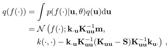
Here, \(M\) is the number of inducing points. The quality of the model depends almost entirely on \(M\).

• Low \(M\): The model is fast but blurry; it misses details.
• High \(M\): The model is accurate but slow and memory-hungry.

In standard approaches, \(M\) is a fixed hyperparameter chosen by the human. The goal of this research is to make \(M\) dynamic.

VIPS: A “Las Vegas” Algorithm for Model Sizing

The researchers propose VIPS (Vegas Inducing Point Selection). The name is a nod to “Las Vegas Algorithms”—randomized algorithms that always produce a correct result (satisfying a specific condition), though the time it takes to do so may vary.

The core idea of VIPS is simple yet profound: Keep adding inducing points until the model is “good enough” compared to the theoretically optimal model.

The Theoretical Gap

To determine if the model is good enough, we need a metric. In Bayesian inference, we often maximize the ELBO (Evidence Lower Bound). The ELBO balances data fit against model complexity.

The researchers derived a way to measure the gap between the model’s current performance (the lower bound) and the best possible theoretical performance (an upper bound).

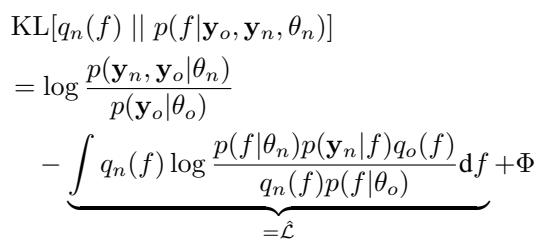
This equation shows the Kullback-Leibler (KL) divergence, which measures how far our approximation is from the true posterior distribution. We can’t calculate the true posterior exactly, but we can bound the error.

The Algorithm

The VIPS algorithm operates on every new batch of data that arrives. It follows a greedy process:

1. Assess: Calculate the current Lower Bound (how well we are doing) and the Upper Bound (how well we could possibly do).
2. Check: Is the gap between them small enough?
3. Act: If the gap is too large, find the data point in the current batch that the model is most “confused” about (highest variance). Turn that data point into a new inducing point.
4. Repeat: Recalculate and repeat until the gap closes.

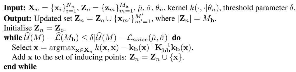
This method ensures that we only add capacity when the model actually struggles to represent the new data. If the new data is redundant (similar to what we’ve seen before), the gap will be small, and the model size won’t grow.

The Stopping Threshold

The critical question is: What is the threshold? If we set the tolerance too tight, the model will keep adding points until it essentially memorizes the dataset (overfitting and growing too large).

The authors propose a threshold relative to a noise model. We want to capture a high proportion of the information in the signal, but we don’t need to model the random noise.

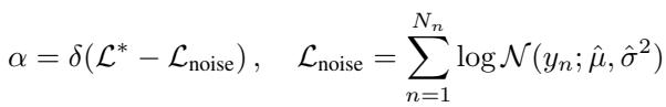
By setting the threshold \(\alpha\) based on the noise level of the data, the method becomes robust. It works for datasets with high signal-to-noise ratios and those with lots of noise, without requiring manual tuning for every new problem.

Visualizing Adaptive Growth

To see VIPS in action, let’s look at three different synthetic scenarios. This visualization perfectly illustrates why a “one-size-fits-all” fixed model fails.

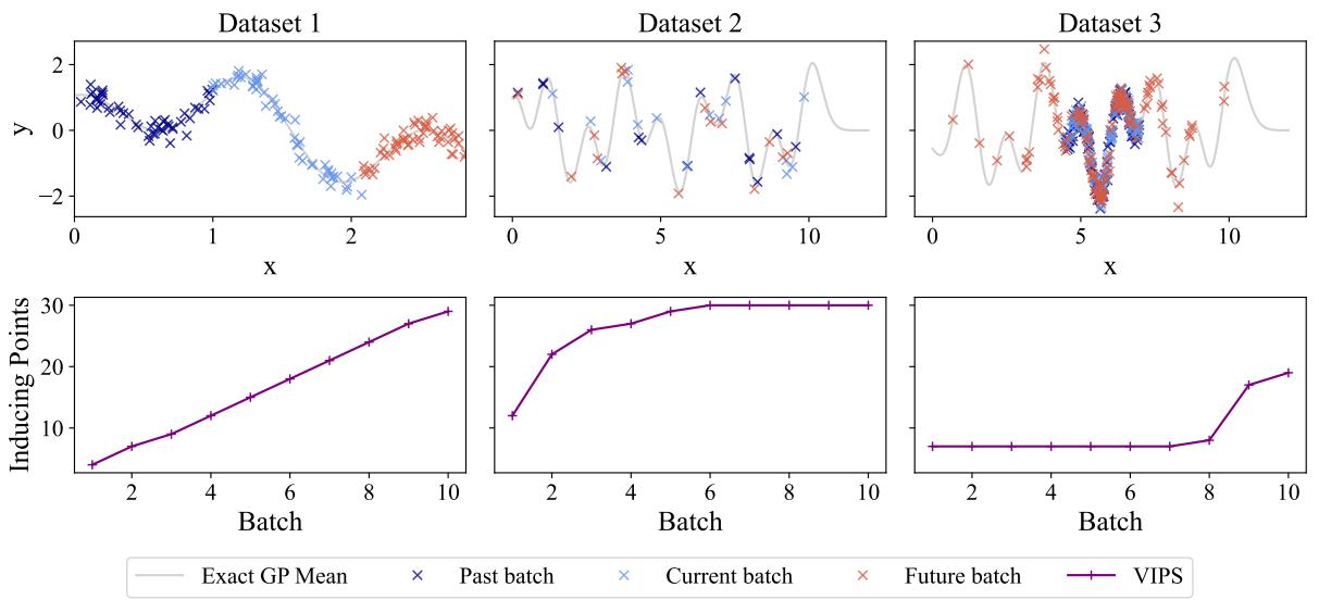
1. Scenario 1 (Left): The input space keeps growing (the x-axis expands). The model encounters constantly novel data. VIPS responds by linearly increasing the number of inducing points. A fixed model would have run out of capacity halfway through.
2. Scenario 2 (Middle): The data comes from the same region over and over. After the initial learning phase, the new data doesn’t add much “novelty.” VIPS correctly identifies this and halts growth, saving computation. A heuristic that adds “10 points per batch” would have been wasteful here.
3. Scenario 3 (Right): The data is mostly simple, but occasionally, outliers (red crosses) appear in new regions. VIPS keeps the model small during the simple phases but spikes in size immediately when it needs to capture the outliers.

Experimental Results

Does this theory hold up against benchmarks and real-world tasks? The researchers compared VIPS against fixed-size methods and other adaptive algorithms (like “Conditional Variance” or CV, and OIPS).

Fixed vs. Adaptive

First, let’s look at the risk of guessing a fixed size.

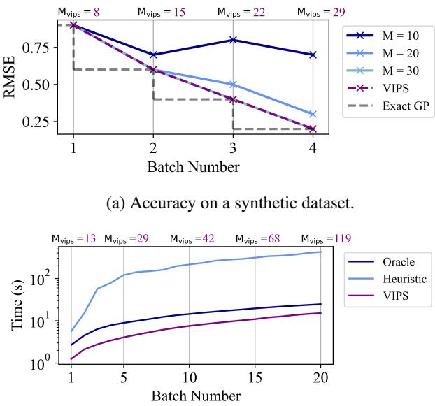
In Figure 2(a), notice the blue lines. If you pick \(M=10\) or \(M=20\) (fixed sizes), the error (RMSE) improves for a while but then plateaus or gets worse because the model is “full.” The purple line (VIPS) automatically grows to match the performance of the exact GP (the theoretical ceiling).

In Figure 2(b), look at the training time. An “Oracle” (someone who knew the perfect size beforehand) set \(M=100\). A standard heuristic set \(M=1000\) (just to be safe). VIPS (purple) stays faster than the heuristic and competitive with the Oracle, because it didn’t waste time computing unnecessary parameters in the early batches.

Robustness Across Datasets

A major claim of the paper is that VIPS requires less tuning. In continual learning, you usually can’t tune hyperparameters because you can’t replay the stream. You need a setting that works “out of the box.”

The researchers tested VIPS on several UCI benchmark datasets. They counted how often each method achieved the smallest model size while still meeting a strict accuracy threshold.

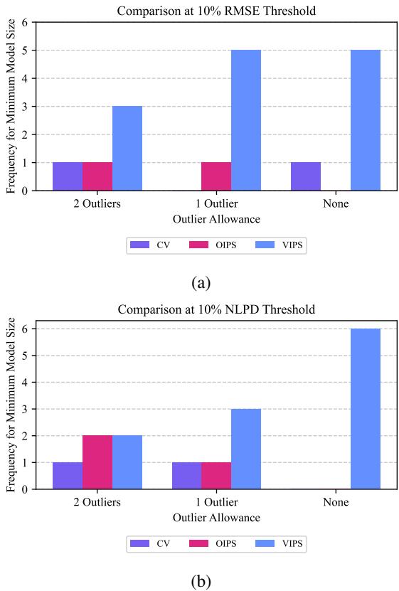
The blue bars represent VIPS. Across different error tolerances (RMSE and NLPD), VIPS consistently achieved the “win”—meaning it found the most efficient model size more often than the competitors (CV and OIPS). This suggests VIPS is safer to use when you don’t know the dataset characteristics in advance.

Real-World Application: Robot Mapping

The most compelling demonstration involves a robot exploring a room to map magnetic field anomalies. This is a classic continual learning setup: the robot drives, collects data, and updates its map. It doesn’t know how complex the magnetic field is until it gets there.

Let’s look at the map generated by VIPS:

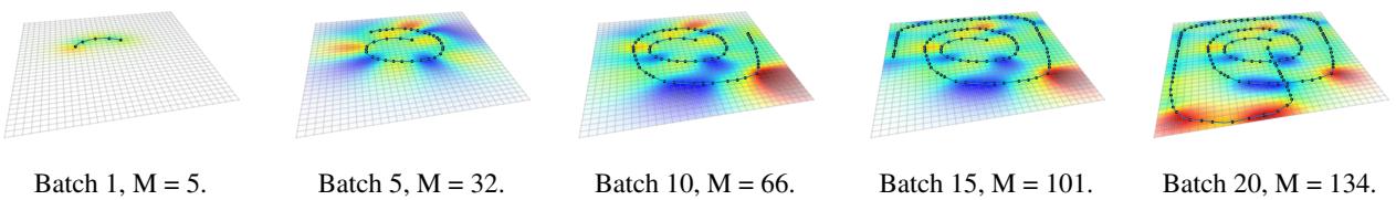
In Figure 8, the black dots represent the inducing points selected by VIPS. Notice how the number of points (\(M\)) grows steadily from 5 to 134 as the robot drives a complex path. The model places points densely where the path twists and turns (high complexity) and sparsely where the path is straight.

Now, compare this to a competitor method, Conditional Variance (CV):

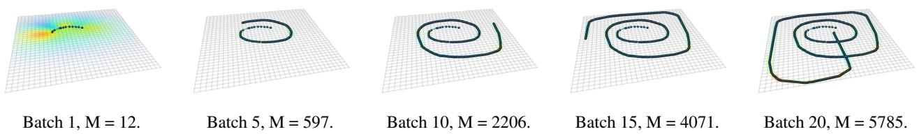
In Figure 10, the Conditional Variance method explodes in complexity. By batch 20, it has selected 5,785 inducing points! This is computationally disastrous for a small robot. It added points everywhere, regardless of necessity.

On the other extreme, let’s look at OIPS:

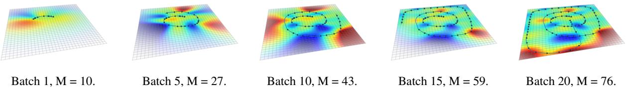
In Figure 12, OIPS is too conservative. It only selects 76 points. While efficient, previous benchmarks in the paper showed that OIPS often fails to meet accuracy thresholds because it stops growing too early.

VIPS strikes the “Goldilocks” balance: enough points to be accurate (like the full GP), but few enough to be computationally viable on a robot.

Conclusion

The question “How big is big enough?” is central to efficient machine learning. This research provides a principled answer for Gaussian Processes. By mathematically bounding the difference between the current approximation and the optimal solution, VIPS allows models to self-regulate their size.

Key takeaways:

1. Efficiency: VIPS grows linearly when learning new concepts but plateaus when data becomes repetitive.
2. Safety: Unlike heuristics, it has a theoretical guarantee regarding the approximation quality.
3. Practicality: It performs well across diverse datasets with a single hyperparameter, solving a major pain point in streaming data where tuning is impossible.

While this paper focuses on Gaussian Processes, the principles of separating model capacity from approximation quality offer exciting directions for the broader field of deep learning. As we move toward AI agents that learn continuously in the real world, adaptive capacity methods like VIPS will be essential to keep them smart without burning out their processors.