](https://deep-paper.org/en/paper/11083_learning_dynamics_in_lin-1818/images/cover.png)
Recurrent Neural Networks (RNNs) are the workhorses of temporal computing. From the resurgence of state-space models like Mamba in modern machine learning to modeling cognitive dynamics in neuroscience, RNNs are everywhere. We know that they work—they can capture dependencies over time, integrate information, and model dynamic systems. But there is a glaring gap in our understanding: we don’t really know how they learn.
Most theoretical analysis of RNNs looks at the model after training is complete. This is akin to trying to understand how a skyscraper was built by only looking at the finished building. To truly understand the emergence of intelligence—artificial or biological—we need to look at the construction process itself: the learning dynamics.
In a recent paper titled “Learning dynamics in linear recurrent neural networks”, researchers Proca, Dominé, Shanahan, and Mediano provide a breakthrough analytical framework. By focusing on Linear RNNs (LRNNs), they strip away the noise of non-linearities to reveal the fundamental mathematical principles governing how these networks learn from time-dependent data.
This post will take you through their derivation, uncovering why RNNs learn some things faster than others, why they sometimes become unstable, and how the very nature of recurrence forces a network to learn rich features rather than lazy shortcuts.
The Setup: Defining the Linear RNN
To analyze learning dynamics mathematically, we need a tractable model. The authors focus on a Linear RNN. While it lacks the activation functions (like ReLU or Tanh) of deep networks, it retains the core structural element: the hidden state that evolves over time.
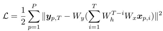
The model is defined by a hidden state \(h_t\) that updates based on its previous state and a new input \(x_t\), and finally produces an output \(\hat{y}\).
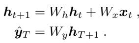
If we unroll this recurrence over time, we see that the hidden state at any point is a sum of all previous inputs, weighted by powers of the recurrent matrix \(W_h\). This exponentiation (\(W_h^{t-i}\)) is the key feature of RNNs—it is how the network travels through time.
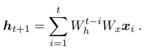
The network is trained to minimize the squared error between its prediction and the target. This loss function sums over all trajectories \(P\) in the dataset.
Task Dynamics
The crucial innovation in this paper is how the authors define the “task.” In linear networks, the task is defined by the statistical relationship between inputs and outputs. The authors introduce the concept of Task Dynamics.
Instead of treating the data as a static blob, they decompose the correlation between the input at time \(t\) and the final output target. They utilize Singular Value Decomposition (SVD) to represent these correlations.
As shown in Figure 1, the input-output correlation matrices are decomposed into singular vectors (\(U_y, V_x\)) and singular values (\(S_t\)). A key assumption here is that the vectors stay constant, but the singular values (\(S_t\)) change over time. This allows the researchers to study how the network learns “temporal structure”—essentially, how the importance of the input changes depending on when it appears in the sequence.
The Core Method: Decoupling the Dynamics
Calculating the gradient descent dynamics for an RNN is notoriously difficult because parameters are shared across all time steps (the same \(W_h\) is used at \(t=1\) and \(t=100\)).
To solve this, the authors assume the network’s weights are “aligned” with the data’s singular vectors. This allows them to diagonalize the matrices. Instead of dealing with massive matrices, the problem breaks down into independent scalar equations for each singular value dimension \(\alpha\).
We can now describe the network using three “connectivity modes” (scalar values representing the strength of connections in that dimension):
- \(a_\alpha\): The input mode (representing \(W_x\)).
- \(b_\alpha\): The recurrent mode (representing \(W_h\)).
- \(c_\alpha\): The output mode (representing \(W_y\)).
Under gradient flow (gradient descent with a small learning rate), the evolution of these modes over training time (\(t_\theta\)) is governed by a set of differential equations:
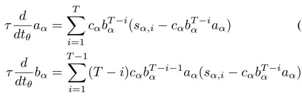
These equations might look intimidating, but they reveal something fascinating. The change in the recurrent mode \(b\) (Equation 6) depends on a term \((T-i)\). This implies that the length of the sequence directly impacts the gradient.
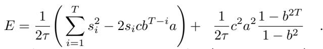
Furthermore, the authors prove that these dynamics are not random; they are effectively minimizing a specific Energy Function:
This energy function (Equation 8) tells us exactly what the network is trying to achieve. It is trying to match the product of its weights (\(c \cdot b^{T-i} \cdot a\)) to the data singular values (\(s_i\)) at every time step \(i\).
Insight 1: Time and Scale Determine Learning Speed
In standard feedforward networks, we know that “larger” singular values are learned first. If a feature explains a lot of variance in the data, the network picks it up quickly.
In RNNs, the story is more complex. The authors found that learning is ordered by scale AND temporal precedence.
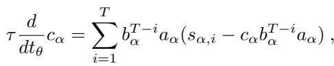
To understand this, they decomposed the data singular values into a constant scaling factor (\(\delta\)) and a time-dependent function \(f(\lambda, t)\).
- Input-Output modes (\(a, c\)) generally learn the constant scaling (\(\delta\)).
- Recurrent modes (\(b\)) learn the time-dependent dynamics (\(\lambda\)).
As seen in Figure 2, the theory (dashed lines) perfectly predicts the simulation (solid lines).
- Left Plot: The input-output modes simply grow to match the scale of the data. Larger \(\delta\) (orange line) learns faster.
- Right Plot: The recurrent modes learn the temporal structure.
Crucially, the authors discovered a Recency Bias. Singular values that are larger and occur later in the sequence are learned faster. This is because the recurrent weight \(b\) acts as a multiplier. If \(b\) starts small (near 0), gradients from early time steps are crushed (vanish) before they affect the update, while gradients from recent time steps remain strong.
Insight 2: Stability and Extrapolation
One of the biggest headaches in training RNNs is stability—avoiding exploding gradients. The analytical framework provides a precise explanation for why some tasks are inherently unstable.
The researchers analyzed three specific types of “Task Dynamics”:
- Constant: Every input is equally important (\(f(\lambda, t) = 1\)).
- Inverse-Exponential: Importance grows over time (\(f(\lambda, t) = \lambda^{T-t}\)). This is “Late-Importance.”
- Exponential: Importance decays over time (\(f(\lambda, t) = \lambda^t\)). This is “Early-Importance.”
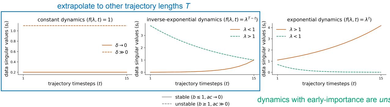
Figure 3 illustrates the consequences of these dynamics:
- Stable (Middle Plot, Orange): When the task has “Late-Importance” (recent inputs matter most), the network learns a recurrent weight \(b \le 1\). This is stable.
- Unstable (Right Plot, Orange): When the task has “Early-Importance” (inputs from long ago matter most), the network must learn a recurrent weight \(b > 1\) to amplify those old signals. This leads to exploding gradients and numerical instability.
The Extrapolation Trap This analysis also explains why RNNs fail to extrapolate. Look at the note in Figure 3 regarding exponential dynamics. The optimal solution for the input-output modes (\(ac\)) depends on the sequence length \(T\).
\[ac = \delta \lambda^T\]If you train the network on sequences of length \(T=10\), it learns a specific value for \(ac\). If you then test it on \(T=20\), the network fails because its learned weights are hard-coded for length 10. The architecture of the RNN (which assumes time-invariant dynamics) fundamentally clashes with tasks where the scale depends on the sequence duration.
Insight 3: The Phase Transition
Real-world data is rarely perfect. What happens when the RNN cannot perfectly fit the data? What if the task requires a mix of “remembering the past” (recurrent) and “looking at the present” (feedforward)?
The authors rewrote the energy function to reveal a hidden interaction:
Equation 9 highlights an Effective Regularization Term. This term punishes large weights, specifically pushing the recurrent mode \(b\) toward zero.
This creates a tug-of-war. The data wants the network to learn the dynamics (increasing \(b\)), but this regularization term wants to keep the network simple (keeping \(b\) small). This leads to a Phase Transition.
To demonstrate this, the authors created a synthetic task with a “feedforward” component (\(\kappa\)) at the last step and a “recurrent” component determined by singular values \(s_t\).
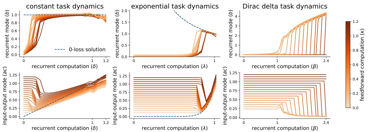
Figure 4 shows this dramatic behavior.
- Left Side of plots: When the recurrent computation is weak (low X-axis value), the network effectively gives up on recurrence. It sets \(b \approx 0\) and uses the input-output weights to just fit the final timestep. It acts like a feedforward network.
- Right Side of plots: As the recurrent information becomes strong enough, the network suddenly snaps into a different mode. \(b\) jumps up, and the network begins to model the full sequence.
This suggests that RNNs have an implicit bias toward low-rank, simple solutions. Unless the temporal data is strong enough to overcome the regularization, the network will prune its own recurrent dynamics.
Insight 4: Recurrence Forces Feature Learning
In the world of deep learning theory, there is a distinction between “Lazy Learning” (where weights barely move and the network acts like a kernel machine) and “Rich Learning” (where the network learns useful features).
Feedforward linear networks can often be “lazy.” But does recurrence change this?
The authors derived the Neural Tangent Kernel (NTK) for their LRNN. The NTK describes how the network evolves. If the NTK is constant, the learning is lazy. If the NTK moves, the learning is rich.
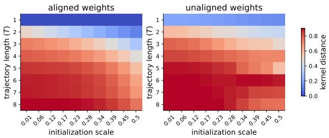
Figure 5 compares the change in the NTK (Kernel Distance) for different trajectory lengths (\(T\)).
- T=1 (Bottom rows): This is essentially a feedforward network. The kernel distance is low (blue).
- T=8 (Top rows): As the sequence length increases, the kernel distance turns red (high movement).
This proves that recurrence encourages feature learning. The repeated application of the same weight matrix \(W_h\) amplifies small changes, forcing the network out of the lazy regime and compelling it to learn structured representations.
Validation: The Sensory Integration Task
To prove these theoretical insights aren’t just mathematical curiosities, the authors applied them to a “Sensory Integration” task common in neuroscience. The network receives noisy inputs and must output either the Mean or the Sum of the inputs.
- Sum Integration: This implies constant dynamics (\(y = \sum x\)). The ideal recurrent weight is \(b=1\), and input-output weights should be \(1\). This solution is independent of \(T\).
- Mean Integration: This requires scaling by \(1/T\). The input-output weights depend on the sequence length.
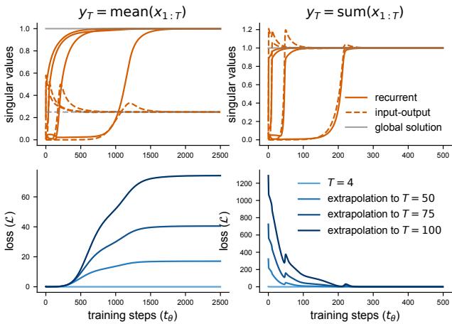
The results in Figure 6 confirm the theory:
- Top Row: The singular values converge exactly where the theory predicts (orange lines matching the gray global solution).
- Bottom Row:
- Sum (Right): The network extrapolates perfectly. The loss remains near zero even as \(T\) changes.
- Mean (Left): The network fails to extrapolate. Because it learned a specific scaling for the training length, it cannot handle new lengths.
Conclusion
We often treat Neural Networks as black boxes, but Proca et al. demonstrate that we can crack them open—at least the linear ones. By treating the learning process as a dynamic system itself, they revealed that RNNs are not neutral observers of time. They have biases. They prefer recent events. They struggle with long-term dependencies that fade into the past. And they have an inherent pressure to simplify their own connectivity.
These insights help explain why RNNs behave the way they do, bridging the gap between abstract machine learning theory and the dynamical systems observed in biological neuroscience. As we push toward more complex architectures, understanding these fundamental dynamics of learning is the key to building models that don’t just memorize data, but truly understand time.