Introduction

Clustering is one of the most intuitive tasks in data analysis. We look at a pile of data points—be they images, documents, or biological samples—and try to group similar items together while keeping dissimilar items apart. But what happens when “similarity” isn’t enough?

Imagine you are clustering news articles. An algorithm might group two articles because they share keywords. However, you, the human expert, know for a fact that one article is about the 2024 Olympics and the other is about the 2028 Olympics. You want to enforce a hard rule: these two must strictly be in different clusters. Conversely, you might have two articles in different languages that describe the exact same event; you want to mandate that they end up in the same cluster.

This is the realm of Constrained Correlation Clustering (CCC). It takes the standard clustering problem and adds “Must-Link” and “Cannot-Link” constraints. While this sounds like a minor tweak, it makes the mathematical problem significantly harder. For years, the best theoretical algorithm for this problem provided a “3-approximation”—meaning the solution found could cost up to three times as much as the perfect, optimal solution.

In standard (unconstrained) correlation clustering, researchers have long since broken the “2-approximation” barrier, achieving much tighter results. But the constrained version has been stuck at 3. Until now.

In the paper “Towards Better-than-2 Approximation for Constrained Correlation Clustering,” researchers Andreas Kalavas, Evangelos Kipouridis, and Nithin Varma present a breakthrough approach. By combining Linear Programming (LP) with a clever “Local Search” technique, they show that—conditional on solving the LP efficiently—we can achieve an approximation factor of 1.92.

In this post, we will tear down this complex paper. We will explore how they use a fractional solution to guide a discrete search, how they “mix” different clusterings to avoid worst-case scenarios, and how they finally crack the barrier of 2.

Background: The Rules of the Game

Before we dive into the new method, let’s establish the ground rules of Correlation Clustering and why constraints complicate things.

Correlation Clustering

In the standard version of this problem, you are given a complete graph where every pair of nodes (vertices) has an edge labeled either \(+\) (plus) or \(-\) (minus).

• Plus (+): These nodes want to be in the same cluster.
• Minus (-): These nodes want to be in different clusters.

The goal is to partition the nodes into clusters to minimize the Cost, which is the sum of:

1. Minus edges inside clusters (items that hate each other but are forced together).
2. Plus edges between clusters (items that like each other but are separated).

A key feature of Correlation Clustering is that you do not specify the number of clusters (\(k\)) beforehand. The algorithm decides the optimal \(k\) naturally based on the edge labels.

Adding Constraints

The constrained version introduces two sets of hard constraints:

• Friendly Pairs (\(F\)): A set of pairs that must be in the same cluster.
• Hostile Pairs (\(H\)): A set of pairs that must be in different clusters.

You might think, “Can’t we just merge the Friendly pairs into super-nodes and proceed as usual?” Unfortunately, no. Merging nodes creates weighted edges and structural dependencies that standard algorithms aren’t equipped to handle without losing their approximation guarantees. Furthermore, a valid clustering must satisfy all constraints in \(F\) and \(H\). If you have a Friendly pair \((u, v)\) and a Hostile pair \((u, w)\), then \((v, w)\) implicitly becomes hostile. Managing these transitive relationships is tricky.

The Metric: Approximation Factor

Since finding the exact optimal clustering is NP-Hard (computationally impossible for large datasets), we look for approximation algorithms. An algorithm is an \(\alpha\)-approximation if:

\[ \text{Cost(Our Algorithm)} \le \alpha \times \text{Cost(Optimal Solution)} \]

For CCC, the previous best \(\alpha\) was 3. This paper aims for \(\alpha < 2\).

The Core Method

The authors’ approach is a masterclass in hybrid algorithm design. It doesn’t rely on just one technique. Instead, it combines Linear Programming (LP) to get a “fractional” view of the world, and Local Search to turn that fraction into a solid, discrete clustering.

Here is the high-level roadmap of their algorithm:

1. The LP: Solve a massive Linear Program to get a “fractional optimal” solution.
2. Local Search 1: Use the LP to guide a search for a good clustering (\(\mathcal{L}\)).
3. Local Search 2: If \(\mathcal{L}\) isn’t good enough, run a second search (\(\mathcal{L}'\)) that is penalized for being similar to \(\mathcal{L}\).
4. Pivot (The Mix): If both searches fail to break the barrier, combine them with the LP solution to form a third clustering (\(\mathcal{P}\)) that is guaranteed to be good.

Let’s break these down step-by-step.

1. The Constrained Cluster LP

The foundation of this method is a Linear Program (LP). Standard LPs for clustering usually assign a variable \(x_{uv}\) between 0 and 1 representing the “distance” between two nodes (0 = same cluster, 1 = different cluster).

However, the authors use a more powerful formulation called the Cluster LP. Instead of just looking at pairs, they look at potential clusters.

Let \(z_C\) be a variable representing the probability that a specific set of nodes \(C\) forms a cluster. Let \(x_{uv}\) be the derived distance between nodes \(u\) and \(v\).

The LP tries to minimize the cost of disagreements:

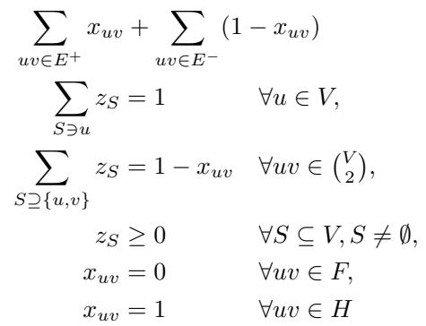
Let’s decode Figure 1 (above):

• Objective: Minimize the sum of distances (\(x_{uv}\)) for plus edges and similarities (\(1-x_{uv}\)) for minus edges. This is the fractional analog of the clustering cost.
• Constraint 1 (\(\sum z_S = 1\)): Every node \(u\) must belong to exactly one cluster distribution (sum of probabilities of clusters containing \(u\) is 1).
• Constraint 2 (\(1 - x_{uv}\)): The probability that \(u\) and \(v\) are in the same cluster is equal to the sum of \(z_S\) for all clusters \(S\) that contain both.
• Hard Constraints: The last two lines are crucial. If a pair is in \(F\) (Friendly), their distance \(x_{uv}\) is forced to 0. If in \(H\) (Hostile), it is forced to 1.

The Assumption: The authors assume we can solve this LP efficiently. While the number of potential clusters \(C\) is exponential, for unconstrained clustering, we know how to solve this in polynomial time. The authors posit that this is likely possible for the constrained version too, or that we can get close enough. The rest of the paper assumes we have this solution.

2. Local Search: The First Pass

Now that we have a fractional solution (a list of clusters \(C\) with weights \(z_C > 0\)), we need an actual clustering. The authors use a Local Search strategy.

How Local Search Works

1. Start with any valid clustering that satisfies the hard constraints.
2. Look at the “good” clusters identified by the LP (those where \(z_C > 0\)).
3. Pick a cluster \(C\) from the LP solution.
4. The Move: Check if forcing \(C\) into your current clustering improves the total cost. If you add \(C\), you remove the nodes in \(C\) from their old clusters and group them together. The remaining fragments of the old clusters stay as they are.
5. Repeat until no more single-cluster swaps improve the cost.

Let’s call the resulting clustering \(\mathcal{L}\).

The authors prove a powerful bound for this simple procedure. They show that the cost of \(\mathcal{L}\) is related to the cost of the LP solution (\(\text{LP}\)) by the following inequality:

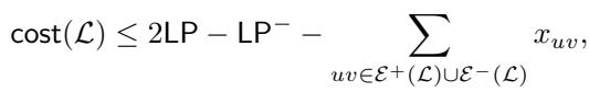
Let’s analyze the image above. It states that the cost of our clustering \(\mathcal{L}\) is at most \(2 \times \text{LP}\). This immediately gives us a 2-approximation!

But look closer at the negative terms. The cost is actually better than \(2 \text{LP}\) by the amount of:

1. \(\text{LP}^-\) (The LP’s cost for minus edges).
2. The distances \(x_{uv}\) of the edges that our clustering \(\mathcal{L}\) fails to satisfy.

This implies that \(\mathcal{L}\) is a strictly better-than-2 approximation unless these subtracted terms are tiny. If \(\mathcal{L}\) is “bad” (i.e., close to factor 2), it implies that specific conditions must be met regarding which edges are satisfied.

Specifically, if \(\mathcal{L}\) is not good enough, it means the LP didn’t pay much for minus edges, and the plus edges we cut had very small \(x_{uv}\) distances in the LP.

3. Local Search with Penalties

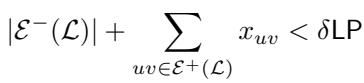
The authors define a small constant \(\delta\) (delta). They aim to prove they can achieve a \((2-\delta)\)-approximation.

From the previous section, if \(\mathcal{L}\) fails to be a \((2-\delta)\)-approximation, we know the “error” is concentrated in a specific way. To counter this, the authors run the Local Search again to produce a second clustering, \(\mathcal{L}'\).

But we don’t want \(\mathcal{L}'\) to make the same mistakes as \(\mathcal{L}\). We want it to be different. So, they modify the cost function for this second search. They add a penalty:

As shown in the image above, the new cost function \(\text{cost}_\mathcal{L}(\mathcal{C})\) is the normal cost plus the number of plus-edges that are unsatisfied in both the new clustering and the old clustering \(\mathcal{L}\).

Intuitively, this forces the algorithm: “Find a low-cost clustering, but try really hard to satisfy the plus-edges that the first clustering failed.”

If this second clustering \(\mathcal{L}'\) is also not better than a 2-approximation, it implies even stricter conditions on the LP solution. We now have two “failed” clusterings, but their failures provide us with structural information about the problem instance.

4. The Pivot: Mixing Everything Together

This is the most innovative part of the paper. We have three ingredients:

1. \(\mathcal{L}\): The result of the first local search.
2. \(\mathcal{L}'\): The result of the penalized local search.
3. \(\mathcal{I}\): A clustering generated by randomly rounding the LP solution (a process called “Sampling”).

If \(\mathcal{L}\) and \(\mathcal{L}'\) are both “bad” (close to 2-approximation), the authors construct a new clustering \(\mathcal{P}\) by mixing these three.

The Labeling System

To build \(\mathcal{P}\), they assign every node \(u\) a label consisting of three coordinates \((X, Y, Z)\):

• \(X\): The cluster containing \(u\) in clustering \(\mathcal{L}\).
• \(Y\): The cluster containing \(u\) in clustering \(\mathcal{L}'\).
• \(Z\): The cluster containing \(u\) in clustering \(\mathcal{I}\).

The algorithm then groups nodes based on these labels.

• Nodes with the exact same label \((X, Y, Z)\) form the core of a new cluster.
• Nodes that differ by only one coordinate are absorbed into these cores.

Why does this work? The authors define a “Pivoting Procedure” (Algorithm 4 in the paper). The logic relies on the assumption that \(\mathcal{L}\) and \(\mathcal{L}'\) were bad. If they were bad, they must have failed to satisfy different sets of edges (because of the penalty). By combining them with the LP-rounded solution \(\mathcal{I}\), the new clustering \(\mathcal{P}\) captures the edges that the others missed.

Experiments & Results: The Theoretical Proof

In theoretical computer science papers, “results” often refer to mathematical proofs rather than benchmarks on datasets. The authors provide a rigorous proof by contradiction.

The Logic: Assume that neither \(\mathcal{L}\) nor \(\mathcal{L}'\) achieves the \((2-\delta)\) approximation.

Step 1: Analyze the “Bad” \(\mathcal{L}\) If \(\mathcal{L}\) is bad, the LP cost must satisfy certain bounds. Specifically, the “minus” edge cost in the LP must be small, and the “plus” edges cut by \(\mathcal{L}\) must have low LP weights.

Step 2: Analyze the “Bad” \(\mathcal{L}'\) If \(\mathcal{L}'\) is also bad, we get a similar inequality, but it includes the intersection of errors with \(\mathcal{L}\).

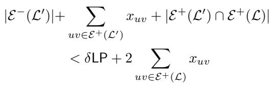
Step 3: The Combined Bound Adding these conditions together tells us that the total weight of edges causing problems is actually quite small relative to the LP cost.

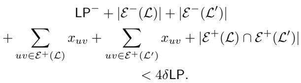
This image essentially says: “If both local searches failed, the total weight of all the ‘problematic’ edges across all solutions is less than \(4\delta \text{LP}\).”

Step 4: The Construction of \(\mathcal{P}\) The authors verify the cost of the third clustering \(\mathcal{P}\).

• If \(\mathcal{P}\) pays for a minus edge, it means the endpoints differed in at most two label coordinates (so \(\mathcal{L}\), \(\mathcal{L}'\), or \(\mathcal{I}\) paid for it).
• If \(\mathcal{P}\) pays for a plus edge, the endpoints differed in at least two coordinates.

Because the total “badness” of \(\mathcal{L}\), \(\mathcal{L}'\), and \(\mathcal{I}\) is bounded (as shown in Step 3), the cost of \(\mathcal{P}\) must also be low.

The Conclusion: The math shows that if we set \(\delta \approx 0.08\), then in the worst-case scenario where \(\mathcal{L}\) and \(\mathcal{L}'\) fail, \(\mathcal{P}\) succeeds.

Specifically, the authors prove that the algorithm always returns a solution with cost at most \((1.92 + \varepsilon) \text{LP}\).

Conclusion and Implications

For nearly two decades, Constrained Correlation Clustering was stuck with a 3-approximation. This paper represents a significant leap forward, bringing the approximation factor down to 1.92.

Key Takeaways:

1. Constraints change the game: You cannot simply “merge and run” standard algorithms. The constraints require handling geometric dependencies.
2. LPs are powerful guides: Even if we can’t use the fractional LP solution directly, it serves as a map. It tells us which clusters are “natural” candidates.
3. Redundancy helps: Running the algorithm twice—once normally, and once with a penalty to force diversity—exposes the structural weaknesses of the problem instance.
4. Mixing solutions: The idea of “pivoting” or mixing multiple clusterings based on node labels is a powerful technique for constructing high-quality solutions from imperfect ones.

The Catch: The result relies on the assumption that the Constrained Cluster LP can be solved (or approximated) efficiently. While this is true for the unconstrained version, and the authors provide strong arguments for why it should hold here, it remains the final hurdle to a fully polynomial-time implementation.

Nonetheless, this work provides the theoretical blueprint for breaking the barrier of 2. It bridges the gap between the messy reality of constrained data and the elegant world of approximation algorithms. For students and researchers in machine learning, it highlights that sometimes, to solve a discrete problem, you have to look at it fractionally, then locally, and finally, mix it all together.

---