The intersection of Artificial Intelligence and Biology has produced some of the most remarkable scientific breakthroughs of the last decade. Tools like AlphaFold have solved the protein structure prediction problem, and Protein Language Models (pLMs) can now generate novel proteins or predict function with uncanny accuracy.

However, there is a catch. While these models are incredibly useful, they function largely as “black boxes.” We feed a sequence of amino acids into the model, and it outputs a structure or a function prediction. But how does it do it? Does the model actually “understand” biophysics, or is it simply memorizing statistical correlations?

If we could peer inside these models, we wouldn’t just understand the AI better; we might discover new biology. This concept is the driving force behind a new paper titled “From Mechanistic Interpretability to Mechanistic Biology,” which applies a technique called Sparse Autoencoders (SAEs) to the ESM-2 protein language model.

This article walks through the researchers’ methodology, their findings on how AI represents protein “concepts,” and how this technology enables us to use AI not just for prediction, but for biological discovery.

1. The Interpretability Gap in Protein Models

To understand the significance of this work, we must first look at the state of Protein Language Models (pLMs). Models like ESM-2 are trained on millions of protein sequences using a “masked token prediction” task. Much like ChatGPT learns to predict the next word in a sentence, ESM-2 learns to predict missing amino acids in a sequence.

In the process of minimizing prediction error, the model learns internal representations (vectors of numbers) that capture deep insights about protein structure and function. Biologists use these representations for downstream tasks, such as predicting whether a protein is thermostable or where it resides in a cell.

However, the internal representations are “dense” and “polysemantic.” A single neuron in the model might activate for multiple, unrelated concepts—perhaps firing for both a hydrophobic helix and a specific binding site. This entanglement makes it nearly impossible to look at a specific neuron and say, “This neuron represents an alpha helix.”

This is where Mechanistic Interpretability comes in. It is a field dedicated to reverse-engineering neural networks. Recently, researchers in Large Language Models (LLMs) have had success using Sparse Autoencoders (SAEs) to decompose these dense representations into “sparse,” interpretable features. The authors of this paper asked: Can we do the same for the language of proteins?

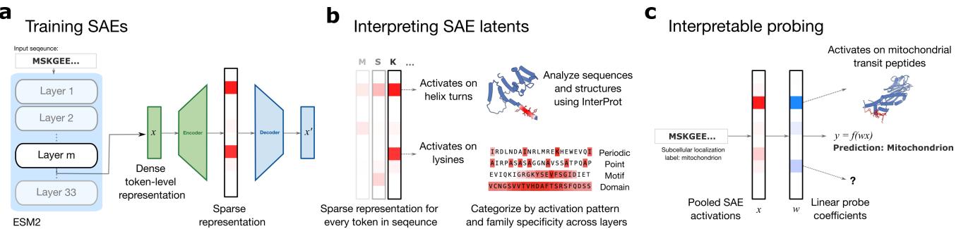
2. The Core Method: Sparse Autoencoders (SAEs)

The goal of an SAE is to take the messy, entangled activations of the pLM and map them into a larger, clearer dictionary of features.

The Architecture

The researchers trained SAEs on the “residual stream” (the main information highway) of various layers of the ESM-2 model (specifically the 650M parameter version).

The SAE architecture consists of two main parts: an Encoder and a Decoder.

The Encoder takes the activation vector \(x\) from the ESM-2 model and projects it into a much higher-dimensional space. The crucial component here is the “TopK” activation function.

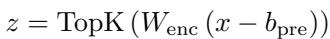
In this equation:

• \(x\) is the input from ESM-2.
• \(W_{enc}\) is the learned weight matrix.
• TopK is the sparsity enforcer. It forces all activations to zero except for the \(k\) highest values.

This constraint forces the model to choose only the most relevant “words” from its dictionary to describe the input protein. By forcing the representation to be sparse, the model is pressured to learn distinct, meaningful features rather than distributed, messy ones.

The Decoder then tries to reconstruct the original input from this sparse representation (\(z\)).

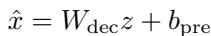
The model minimizes the reconstruction error (the difference between \(x\) and \(\hat{x}\)). If the SAE can accurately reconstruct the ESM-2 activity using only a few active latent dimensions, it implies those dimensions represent the fundamental building blocks (or features) ESM-2 uses to understand proteins.

3. Visualizing the Hidden Language of Proteins

After training the SAEs, the researchers ended up with millions of “latents” (features). The next challenge was interpretation. Unlike English text, where you can read the output, protein sequences are cryptic strings of letters.

To solve this, the authors developed InterProt, a visualization tool. By analyzing which sequences activated specific SAE latents, they could map these mathematical features to biological structures.

The results were striking. The SAE successfully decomposed the model’s knowledge into recognizable biological concepts.

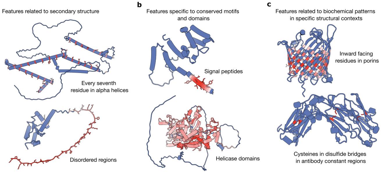
As shown in Figure 2 above, the SAE discovered:

• Secondary Structure (Panel a): Features that specifically light up for alpha helices or disordered regions.
• Motifs and Domains (Panel b): Features that identify signal peptides (which direct protein transport) or specific functional domains like Helicase.
• Biochemical Context (Panel c): Features that detect specific chemical interactions, such as residues involved in disulfide bridges (cysteine-cysteine bonds) or inward-facing residues in a pore.

Human Evaluation

To ensure they weren’t just cherry-picking good examples, the researchers conducted a blinded study. Human experts rated features from the SAE against raw neurons from the ESM model.

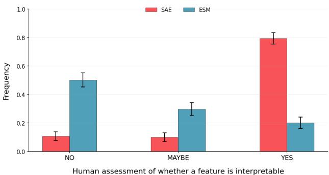
The difference was stark. As Figure 4 shows, roughly 80% of SAE latents were rated as interpretable (“Yes”), compared to a very low percentage for the raw ESM neurons. This confirms that the SAE effectively disentangles biological concepts that are otherwise mixed together in the base model.

4. Protein Families and Layer Dynamics

One of the most fascinating findings of this study is the concept of Family-Specific Features.

The researchers found that many SAE latents are not generic physical detectors (like “alpha helix”). Instead, they are highly specific to evolutionary families. A latent might look for a helix, but only if it appears in a Beta-lactamase enzyme.

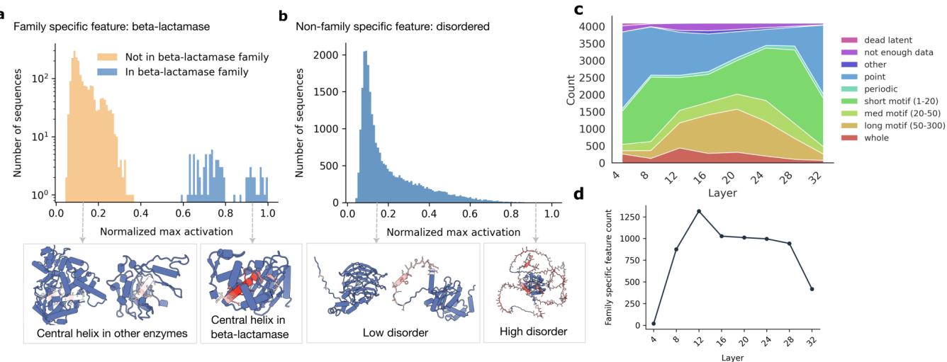
In Figure 3a, we see a latent that activates strongly for the central helix of Beta-lactamase but ignores similar helices in other proteins. Contrast this with Figure 3b, which shows a “disordered” feature that activates broadly across many different protein types.

The Anatomy of Layers

The distribution of these features changes depending on where you look in the model.

• Early Layers: Tend to focus on local amino acid patterns and shorter motifs.
• Middle Layers: This is where family specificity peaks (Figure 3d in the image above). The model seems to group proteins by evolutionary history in these layers.
• Late Layers: The features become more abstract or specialized for the final prediction task.

Classifying Activation Patterns

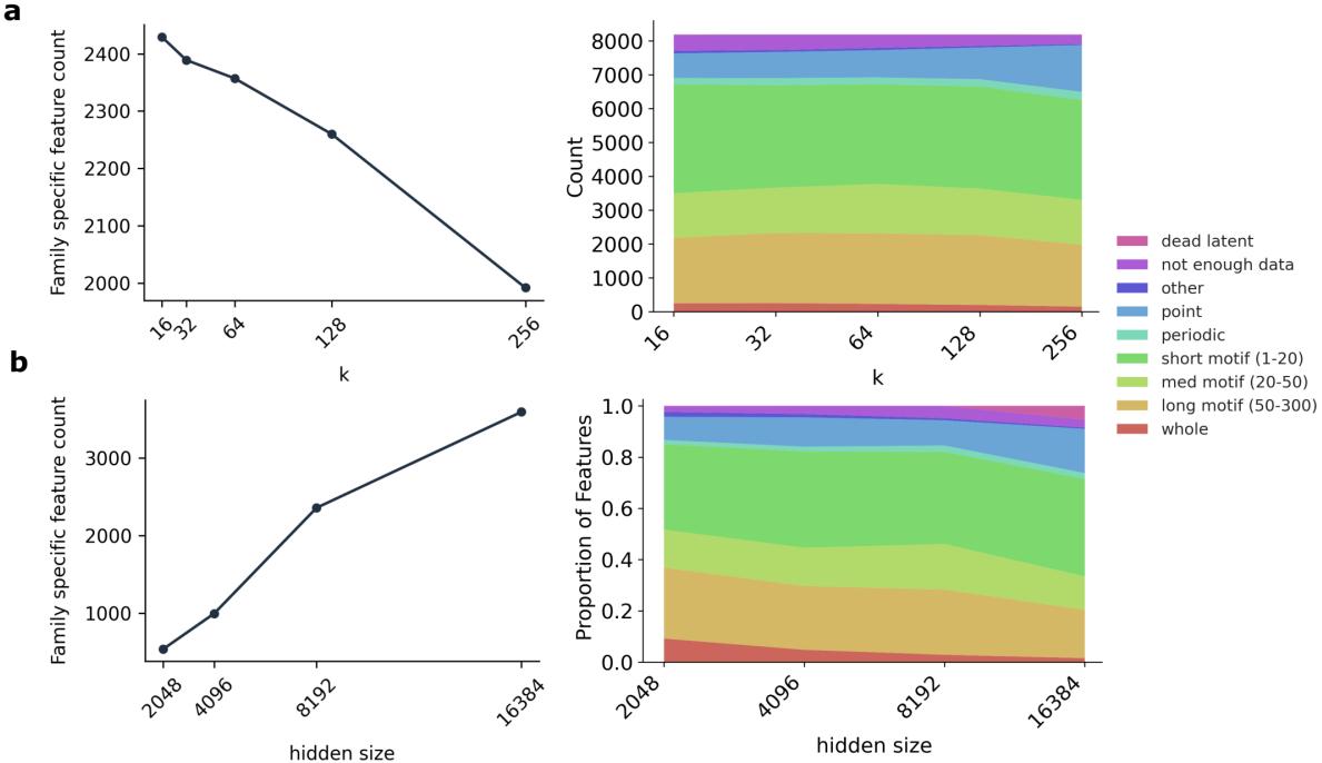
To systematically analyze millions of features, the authors created a classification scheme based on how the features light up along a sequence.

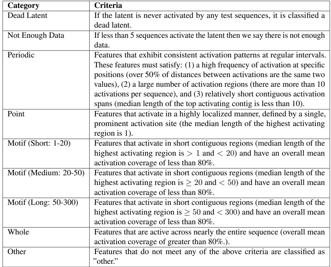
This taxonomy (Table 2) allowed them to quantify how hyperparameters affect feature discovery. For example, they found that increasing the sparsity (lowering \(k\)) forces the model to learn more family-specific features, likely because family identity is a highly efficient way to compress protein information.

5. Interpretable Probing: Connecting Latents to Function

Identifying features is interesting, but can we use them to predict biology? This is where Interpretable Probing comes in.

Standard practice in computational biology is to train a linear classifier (a “probe”) on the output of a pLM to predict properties like subcellular localization. While accurate, these probes are uninterpretable. You get a prediction, but you don’t know why.

The researchers tried a different approach: training linear probes on the SAE latents.

Performance vs. Interpretability

First, they had to ensure that using SAE latents didn’t destroy performance.

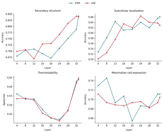
As Figure 5 demonstrates, SAE probes (red lines) perform competitively with standard ESM probes (blue lines) across tasks like Secondary Structure, Subcellular Localization, and Thermostability. In Secondary Structure prediction, the SAE probe actually outperforms the baseline in many layers.

But the real value isn’t the accuracy; it’s the explainability. Because the probe is linear, the researchers could look at the latents with the highest positive weights to understand what biological mechanisms drive the prediction.

Case Study 1: Secondary Structure

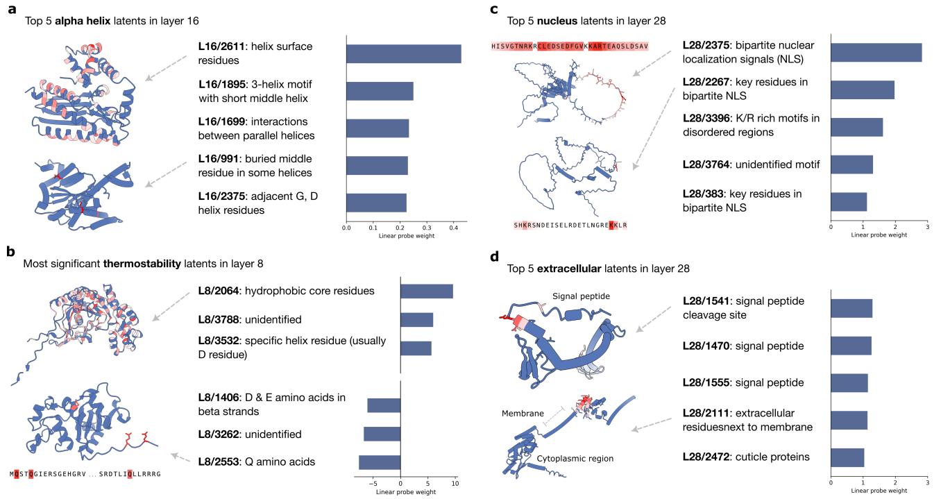
When predicting alpha helices, the probe assigned high weights to latents that explicitly detect helical structures.

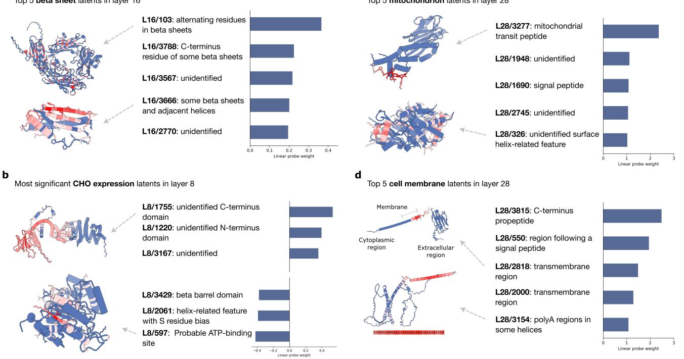
Similarly, for Beta Sheets, the probe found latents that track alternating residue patterns typical of beta-strands.

This confirms that the SAE has learned the “grammar” of protein folding.

Case Study 2: Subcellular Localization

This task involves predicting where a protein goes in the cell (e.g., Nucleus, Mitochondria, Cell Membrane). The biology of this is often driven by “signal peptides”—short sequences that act like shipping labels.

The SAE probes rediscovered these biological mechanisms without supervision.

• Nucleus: The top features (Figure 6c) detect Nuclear Localization Signals (NLS), specifically recognizing the pattern of Arginine (R) and Lysine (K) residues separated by a linker.
• Extracellular/Membrane: The model found features corresponding to Signal Peptides and Transmembrane regions (Figure 9d).

(Note: Figure 9 refers to the mitochondria/membrane panels shown above).

This is a powerful proof of concept: the SAE identified the exact sequence motifs biologists have spent decades characterizing experimentally.

Case Study 3: Thermostability

Predicting how heat-resistant a protein is proved to be a different challenge. Previous research suggested pLMs struggle to scale on this task.

The SAE analysis (Figure 6b) reveals why. The model isn’t learning complex biophysics about protein stability. Instead, the most predictive latents are essentially counting amino acids.

• Positive weights: Hydrophobic core residues (which stabilize proteins).
• Negative weights: Glutamine (Q), which is correlated with instability.

The interpretability of the SAE exposes the model’s strategy: it’s relying on simple composition statistics rather than deep structural understanding for this specific task.

Case Study 4: Mammalian Cell Expression

The researchers also tested a practical industrial task: predicting if a human protein can be successfully expressed in CHO (Chinese Hamster Ovary) cells, which is critical for drug manufacturing.

The SAE found a latent negatively associated with expression that detects an ATP binding site (Figure 9b). This generates a plausible biological hypothesis: perhaps expressing this protein interferes with the host cell’s metabolism by sequestering ATP, causing the expression to fail. This illustrates how SAEs can move from interpretation to hypothesis generation.

Why SAE Probes Work Better for Interpretation

The distribution of the weights in an SAE probe is fundamentally different from a standard probe.

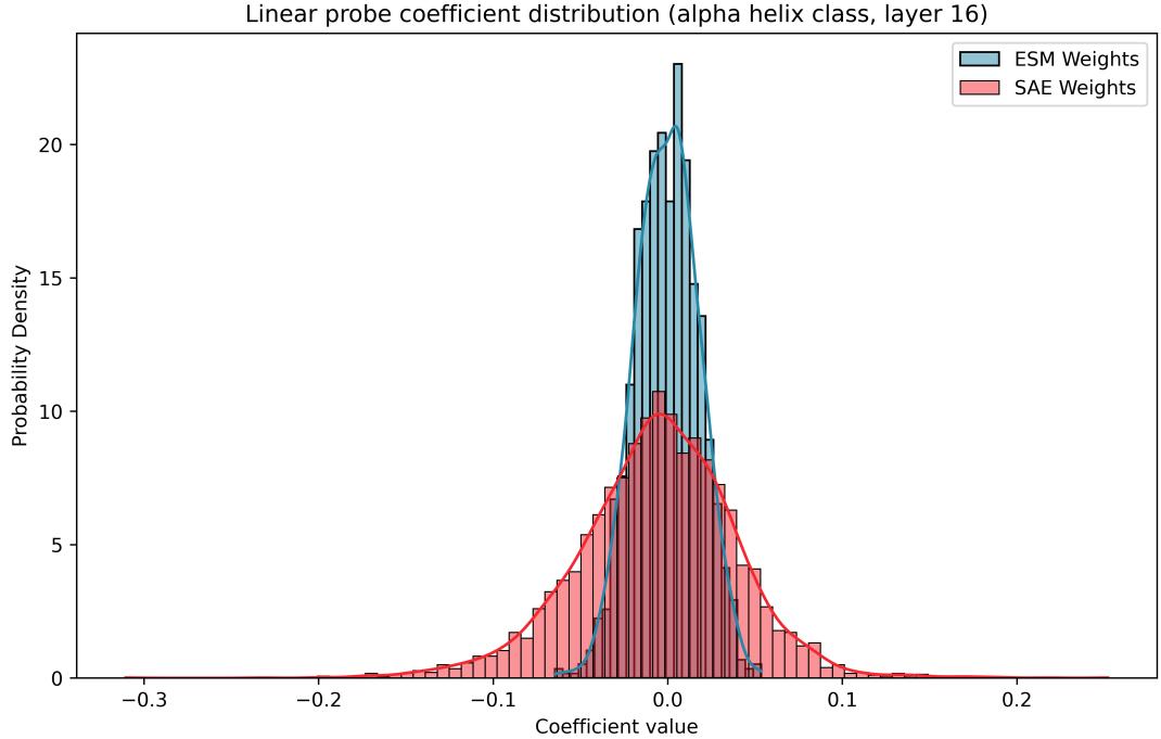
As shown in Figure 10, SAE coefficients (red) have higher variance and a different skew. This indicates that the SAE latents are more “monosemantic”—each one is a distinct predictor—whereas the ESM weights are a messy combination of many small contributions.

6. Validating Features via Steering

The researchers went one step further to validate their “Family-Specific” hypothesis. They performed “steering” experiments, where they artificially clamped the activation of a feature and ran the model to generate sequences.

They compared steering a Family-Specific latent vs. a Random latent.

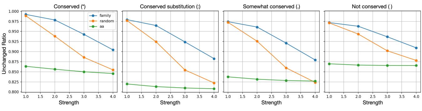
Figure 7 shows the “Unchanged Ratio” of residues. When they steered family-specific latents (blue line), the sequence changed less than when steering random latents, particularly for conserved residues. This suggests that family-specific latents are deeply integrated into the model’s understanding of that protein’s evolutionary constraints.

7. Conclusion: Towards Mechanistic Biology

The transition from “Mechanistic Interpretability” (understanding the model) to “Mechanistic Biology” (understanding life) is the ultimate promise of this technology.

Adams, Bai, and colleagues have demonstrated that Sparse Autoencoders are not just tools for debugging AI. They are microscopes for the high-dimensional data that pLMs learn. By decomposing protein representations into interpretable features, we can:

1. Verify knowledge: Confirm that models use known biology (like NLS motifs) to make predictions.
2. Audit reliability: Detect when models rely on heuristics (like amino acid counting for thermostability) rather than physical principles.
3. Generate hypotheses: Identify predictive features for poorly understood tasks (like CHO expression) to guide experimental biology.

The “black box” of protein language models is beginning to open, revealing a structured, learnable dictionary of biology inside.

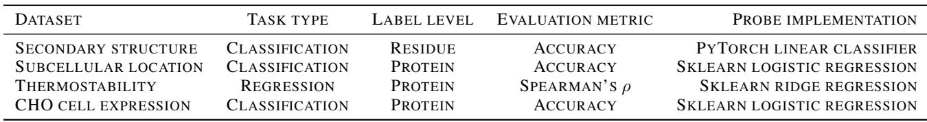
Summary of Downstream Tasks Used: