Introduction: The Paradox of Finding What Isn’t There

Imagine you are a security guard tasked with spotting shoplifters. However, you have never actually seen a shoplifter in your life. You’ve only ever watched honest customers. This is the fundamental problem in Graph-Level Anomaly Detection (GLAD).

In domains like biochemistry (detecting toxic molecules) or social network analysis (identifying bot networks), anomalies are rare, expensive to label, or entirely unknown. Traditional Artificial Intelligence struggles here because standard supervised learning requires examples of both “good” and “bad” data. When you only have “good” data (normal graphs), how do you teach a machine to recognize the “bad”?

For years, researchers relied on reconstruction-based methods: teach a model to draw normal graphs perfectly; if it struggles to draw a new graph, that graph must be an anomaly. But this approach is brittle. Sometimes, anomalies are actually easier to reconstruct than complex normal graphs, leading to failures.

In a recent paper, researchers propose a paradigm shift. Instead of just staring at normal data, what if we used Generative AI to hallucinate our own anomalies?

Enter AGDiff (Anomalous Graph Diffusion). This framework uses Latent Diffusion Models—the same tech behind image generators like Midjourney—not to create perfect images, but to generate “pseudo-anomalous” graphs. By training a detector against these self-generated fakes, AGDiff achieves state-of-the-art performance, effectively teaching itself to spot anomalies by practicing against its own imagination.

The Problem with Existing Methods

Before diving into AGDiff, we need to understand why current methods hit a ceiling.

1. Unsupervised Methods (Reconstruction): These models compress a graph and try to rebuild it. The assumption is that anomalies will have high reconstruction errors. However, this assumes anomalies are structurally complex or vastly different. Subtle anomalies often slip through the cracks.
2. Semi-Supervised Methods: These use a tiny set of labeled anomalies. While effective, they are limited by the specific anomalies provided. If the model learns to spot “Type A” anomalies, it might completely miss a new “Type B” anomaly.

The researchers identified a massive opportunity: Data Augmentation. If we don’t have enough anomalies, we should make them. But random noise isn’t enough; we need “hard” negatives—graphs that look almost normal but contain subtle structural perturbations.

The AGDiff Framework

The core innovation of AGDiff is using a Latent Diffusion Model as a pseudo-anomaly generator.

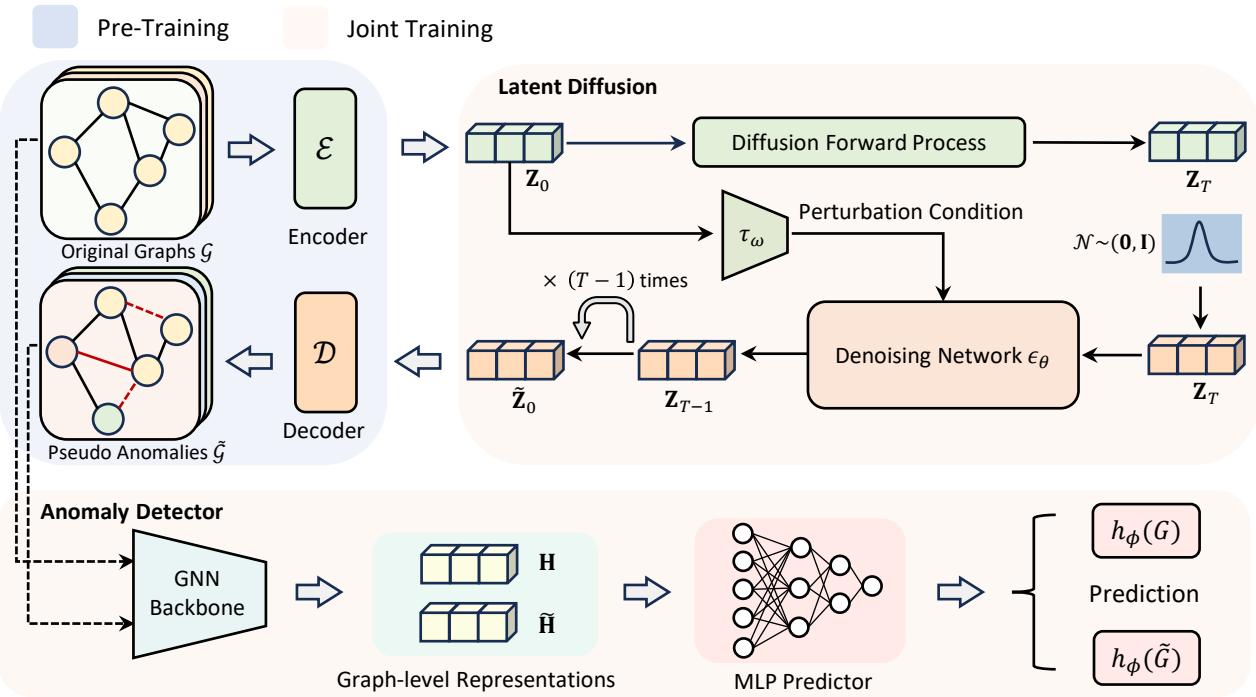
As shown in Figure 1, the architecture is divided into three distinct phases. Let’s break them down.

Phase 1: Pre-Training (Learning Normality)

You cannot effectively break a rule until you understand it. Similarly, AGDiff first needs to understand what a “normal” graph looks like.

The authors use a variational framework (similar to a VAE) to compress graph data (Adjacency matrices \(\mathbf{A}\) and Node features \(\mathbf{X}\)) into a lower-dimensional Latent Space (\(\mathbf{Z}\)).

\[ \begin{array} { r l } & { \mathcal { L } _ { \mathrm { p r e t r a i n } } = \displaystyle \ell _ { \mathrm { r } } ^ { \mathrm { a t t r } } + \ell _ { \mathrm { r } } ^ { \mathrm { e d g e } } + \ell _ { \mathrm { K L } } } \\ & { \quad \quad \quad \quad = \displaystyle \sum _ { i = 1 } ^ { N } ( \| \mathbf { X } _ { i } - \hat { \mathbf { X } } _ { i } \| _ { F } ^ { 2 } + \mathcal { H } ( \mathbf { A } _ { i } , \hat { \mathbf { A } } _ { i } ) } \\ & { \quad \quad \quad \quad - \mathrm { K L } ( q ( \mathbf { Z } _ { i } | \mathbf { X } _ { i } , \mathbf { A } _ { i } ) | \mathcal { P } ( \mathbf { Z } ) ) ) , } \end{array} \]

The pre-training loss (above) ensures that the latent embeddings \(\mathbf{Z}\) capture the essential structural and attribute information of the normal graphs. This latent space serves as the playground for the diffusion model.

Phase 2: Generating Anomalies via Latent Diffusion

This is where AGDiff diverges from standard diffusion applications. Usually, diffusion models are trained to remove noise to generate high-fidelity data. AGDiff uses diffusion to introduce controlled perturbations.

The process happens in the latent space \(\mathbf{Z}\) rather than the graph space. This is computationally efficient and allows for smoother manipulation of graph structures.

The Forward Process

The model progressively adds Gaussian noise to the latent representation of a normal graph over \(T\) timesteps.

\[ \begin{array} { r } { \mathbf { z } _ { t } = \sqrt { \bar { \alpha } _ { t } } \mathbf { z } _ { 0 } + \sqrt { 1 - \bar { \alpha } _ { t } } \epsilon _ { t } , \quad \epsilon _ { t } \sim \mathcal { N } ( \mathbf { 0 } , \mathbf { I } ) , } \end{array} \]

The Conditional Reverse Process

Here is the secret sauce. The authors introduce a Perturbation Condition (\(\mathbf{c}\)). Instead of letting the model reconstruct the original normal graph perfectly, they condition the denoising process on a perturbed vector.

The condition vector \(\mathbf{c}\) is derived from the original latent code \(\mathbf{z}_0\) plus some learnable noise \(\eta\):

\[ \mathbf { c } = \tau _ { \omega } ( \mathbf { z } _ { 0 } ) = \sigma ( \mathbf { W } _ { \mathbf { c } } ( \mathbf { z } _ { 0 } + \boldsymbol { \eta } ) + \mathbf { b } _ { \mathbf { c } } ) , \]

This vector \(\mathbf{c}\) acts as a guide. When the model tries to “denoise” the data, \(\mathbf{c}\) forces it to steer slightly off-course, preventing it from returning exactly to the normal starting point. The reverse diffusion step looks like this:

\[ \mathbf { z } _ { t - 1 } = \frac { 1 } { \sqrt { \alpha } } \left( \mathbf { z } _ { t } - \frac { 1 - \alpha _ { t } } { \sqrt { 1 - \bar { \alpha } _ { t } } } \epsilon _ { \theta } ( \mathbf { z } _ { t } , t , \mathbf { c } ) \right) + \tilde { \beta } \mathbf { v } , \]

The result? A Pseudo-Anomalous Graph. It retains the general structure of the normal graph (because it started from it) but contains subtle distortions introduced by the conditioned diffusion.

Phase 3: Joint Training and Detection

Now the system has a set of Normal Graphs (Real) and a set of Pseudo-Anomalous Graphs (Generated).

The final component is an Anomaly Detector—a binary classifier built on a Graph Isomorphism Network (GIN). The detector is trained to distinguish between the real normal graphs and the generated pseudo-anomalies.

\[ \mathcal { L } = \mathcal { L } _ { \mathrm { c l s } } + \lambda \mathcal { L } _ { \mathrm { d i f f } } \]

The training is a joint process (Equation 14 above). The model simultaneously optimizes the diffusion process (to make realistic but distinct pseudo-anomalies) and the classifier (to tell them apart). This creates a feedback loop:

1. The generator tries to create “hard” anomalies that lie near the boundary of normality.
2. The detector fights to tighten that boundary.
3. The result is a highly discriminative decision boundary that wraps tightly around the normal data.

Why “Generated” Anomalies Beat Reconstruction

You might wonder: Why is training against fake data better than just measuring reconstruction error?

The authors provide a compelling empirical analysis comparing two algorithms:

• \(\mathcal{A}_1\): Reconstruction-based detection.
• \(\mathcal{A}_2\): Discriminative detection using generated pseudo-anomalies (AGDiff).

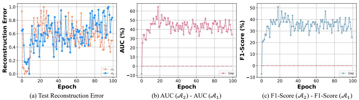
Figure 4 illustrates this dynamic perfectly.

• Graph (a): As training progresses, \(\mathcal{A}_1\) (orange) reduces reconstruction error on normal data. It becomes very good at compression.
• Graph (b): However, look at the AUC gap. \(\mathcal{A}_2\) (blue line) starts outperforming \(\mathcal{A}_1\) significantly as epochs increase.

While \(\mathcal{A}_1\) focuses on compression, it often overfits to the point where it can reconstruct anything, even anomalies. \(\mathcal{A}_2\), by explicitly learning to say “no” to the pseudo-anomalies, learns a much more robust definition of what “normal” actually means.

Experimental Results

The researchers tested AGDiff against comprehensive baselines, including Graph Kernels (like Weisfeiler-Lehman) and modern GNN-based methods (like SIGNET, MUSE, and iGAD). They used two categories of datasets:

1. Moderate-Scale: Molecular graphs (MUTAG, COX2, etc.).
2. Large-Scale Imbalanced: Real-world datasets where anomalies are rare (e.g., SW-620, where only 5.95% of graphs are active compounds).

Performance on Standard Benchmarks

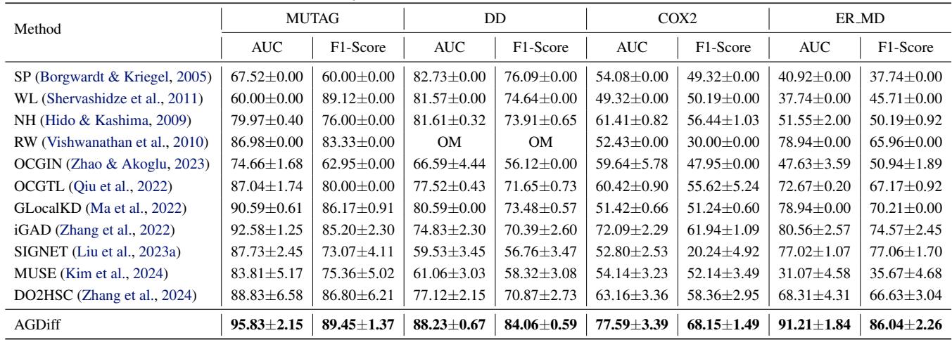
Table 1 shows dominance across the board. On the DD dataset, AGDiff achieves an AUC of 88.23%, smashing the runner-up SIGNET (70.67%) by nearly 18 percentage points. Even compared to semi-supervised methods like iGAD (which actually use real labeled anomalies), AGDiff (which is unsupervised) often wins or performs competitively.

Performance on Imbalanced Data

The real test of an anomaly detector is the “needle in a haystack” scenario.

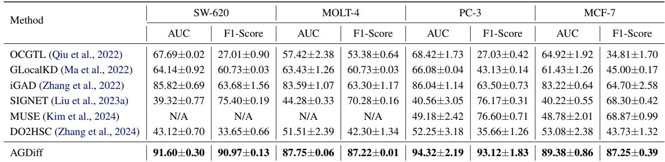
In Table 2, the gap widens. On PC-3, AGDiff hits 94.32% AUC, while the best unsupervised baseline (MUSE) manages only 49.18%. This proves that when data is scarce and imbalanced, generating diverse pseudo-supervision signals is far more effective than relying on the uneven statistics of the dataset itself.

Visualizing the Latent Space

To prove the model isn’t just memorizing data, the authors visualized the latent embeddings using t-SNE.

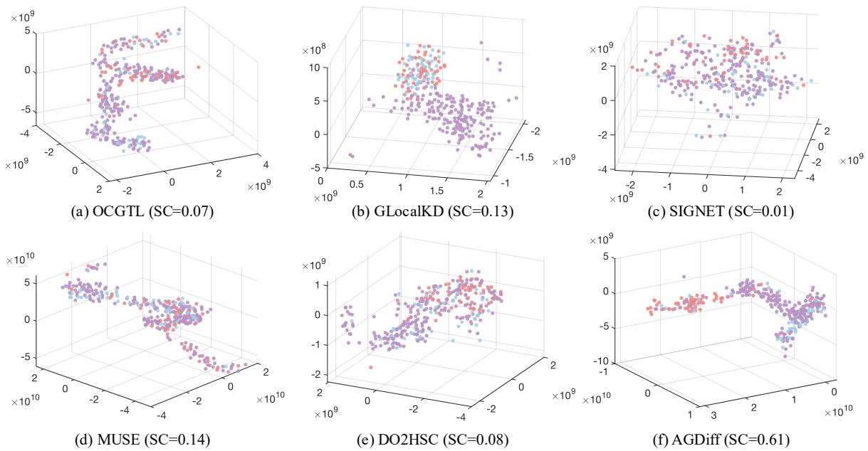
In Figure 5, look at the difference between (f) AGDiff and the others.

• In plots (a) through (e), the red dots (anomalies) are buried inside the purple/blue clusters (normal data). The models are confused.
• In (f), AGDiff has pushed the red dots into a distinct region. The Silhouette Coefficient (SC) jumps to 0.61, far higher than the next best (0.14). This separation is exactly what makes the classification step so accurate.

What Do “Pseudo-Anomalies” Look Like?

It is important to verify that the generated graphs aren’t just random static. They need to look like plausible graphs.

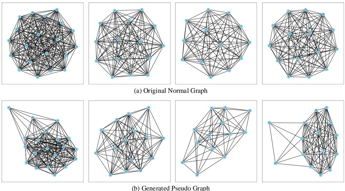
Figure 6 compares original normal graphs (top row) with their generated pseudo-anomalous counterparts (bottom row).

• Structure Preservation: The pseudo-graphs clearly resemble the parents. They aren’t random noise; they look like molecules.
• Subtle Deviation: Notice the connectivity changes. Some clusters are sparser; some edges are rerouted. These are the “subtle perturbations” the authors aimed for—changes small enough to be difficult to detect, forcing the model to learn fine-grained features.

Influence of Hyperparameters

How sensitive is the model? The authors analyzed the parameter \(\lambda\) (lambda), which controls the balance between the classification loss and the diffusion loss.

\[ \mathcal { L } = \mathcal { L } _ { \mathrm { c l s } } + \lambda \mathcal { L } _ { \mathrm { d i f f } } \]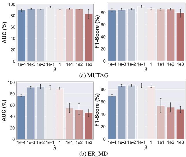

Figure 3 shows a “sweet spot” effect.

• Low \(\lambda\): The model ignores the diffusion quality. The generated anomalies aren’t diverse enough.
• High \(\lambda\): The model focuses too much on diffusion. The pseudo-anomalies might become too similar to normal graphs (over-denoising), confusing the classifier.
• Middle ground: The peak performance occurs where both tasks are balanced.

Conclusion

The AGDiff paper presents a clever inversion of the standard anomaly detection logic. Rather than passively observing normal data and hoping anomalies stand out, AGDiff actively imagines “what could go wrong.”

By leveraging the generative power of Latent Diffusion Models, the framework creates a self-supervised learning environment. It generates diverse, challenging pseudo-anomalies that serve as proxies for the real anomalies we rarely see.

Key Takeaways:

1. Shift to Generation: Moving from reconstruction-based to generation-based detection allows for more robust decision boundaries.
2. Latent Power: Operating in the latent space makes the diffusion process efficient and structurally coherent.
3. Perturbation is Key: The conditional noise injection ensures the generated graphs are useful “near-misses” rather than easy-to-spot garbage.

For students and researchers in Graph Learning, this highlights the growing utility of Diffusion Models beyond just making pretty pictures—they are becoming essential tools for data augmentation and robust representation learning in complex scientific domains.

---