](https://deep-paper.org/en/paper/1703.04813/images/cover.png)
In machine learning, optimization is everything. Whether you’re training a language model, fine-tuning a vision network for self-driving cars, or fitting a simple logistic regression, you’re always using an optimizer—a mathematical engine that nudges your model’s parameters toward better performance.
For decades, the field has relied on meticulously hand-designed optimizers like SGD, ADAM, and RMSProp. These workhorses transformed deep learning by making it possible to train huge networks efficiently.
But what if optimization itself could be learned? Instead of manually designing update rules, could we train a neural network to be the optimizer—to discover its own strategies for navigating loss landscapes? This idea, often called learning to learn or meta-learning, is one of the most enticing directions in modern AI research.
Early attempts were promising but limited. Learned optimizers could perform well on the exact problems they were trained on—but failed to generalize. They were fragile, unable to handle new model architectures or unseen data distributions. Worse, they didn’t scale. Running a separate neural network for every parameter quickly became astronomically expensive.
In the groundbreaking paper “Learned Optimizers that Scale and Generalize” from Google Brain and DeepMind, researchers Olga Wichrowska and colleagues tackled these challenges head-on. They introduced a learned optimizer that not only generalizes to entirely new tasks but can scale to training real-world models like InceptionV3 and ResNetV2 on ImageNet—orders of magnitude larger than anything it saw in training.
This blog post will unpack how they achieved this feat—from architectural innovations to the clever training strategies that gave their optimizer unprecedented flexibility and robustness.
The Limits of Earlier Learned Optimizers
Previous work by Andrychowicz et al. (2016) introduced RNN-based learned optimizers that directly learned how to apply gradient descent. At each step, the RNN received the gradient of a parameter and produced its update.
While elegant, that approach had two fatal flaws:
- Poor Generalization: Optimizers trained on one narrow class of problems—say, small networks with sigmoid activations—often failed spectacularly on even mildly different architectures, like ReLU networks.
- Excessive Overhead: Running one RNN per parameter leads to crushing computational and memory costs. Large-scale models could never be optimized this way.
The work in Wichrowska et al. confronts both issues with a new hierarchical design that scales naturally—and learns behaviors that transfer across problem types.
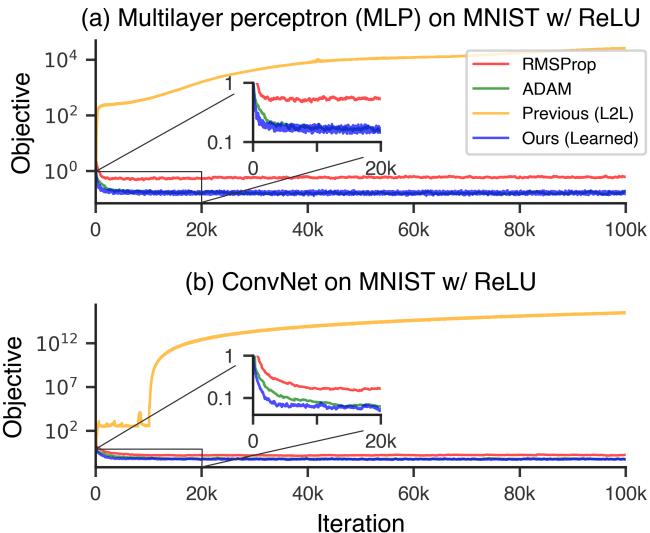
Figure 2. Previous learned optimizers fail on unseen architectures, while the proposed hierarchical optimizer remains stable and effective.
A Smarter Neural Architecture
The centerpiece of the paper is a hierarchical recurrent architecture—a three-level RNN that mirrors the natural structure of neural network parameters.
The Hierarchical Design
Instead of treating every parameter as an independent entity, the optimizer organizes itself around tensors (like weight matrices and bias vectors) and network layers. This drastically reduces overhead while preserving the ability to reason jointly about related parameters.
The hierarchy consists of three levels:
- Parameter RNN (lowest level): A tiny RNN runs for each scalar parameter—just 5–10 hidden units—handling local updates.
- Tensor RNN (middle level): Each parameter tensor (e.g., all weights in a layer) has its own RNN. It aggregates the hidden states of its child Parameter RNNs and sends back a bias signal to coordinate their updates.
- Global RNN (top level): A single RNN processes signals from all tensor-level units, unifying information across the entire network. This allows communication between layers and captures global trends.
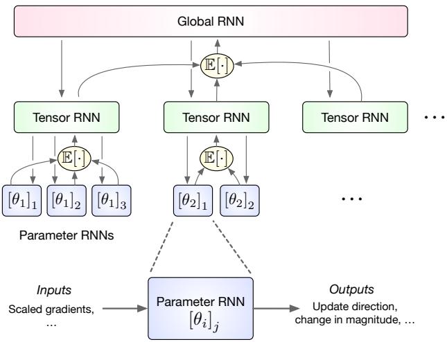
Figure 1. The hierarchical architecture enables coordination across parameters with minimal overhead.
This hierarchy makes the optimizer highly scalable. While each parameter has only a tiny local RNN, the optimizer as a whole communicates structure-aware updates across tensors and layers, capturing interactions that mimic second-order optimization behavior—without exploding in size.
Built-In Optimization Wisdom
Rather than forcing the network to rediscover decades of optimization research entirely from scratch, the authors infused the architecture with inductive biases drawn from classic methods. Four specific features stand out:
1. Looking Ahead: Attention Meets Momentum
Inspired by Nesterov momentum and attention mechanisms, the optimizer sometimes computes gradients not at the current parameter value but at a lookahead position:
\[ \phi_t^{n+1} = \theta_t^n + \Delta \phi_t^n \]This offset allows the network to “peek” ahead in the loss landscape, helping it anticipate curvature and move more confidently toward minima.
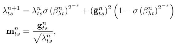
2. Momentum at Multiple Timescales
Standard momentum smooths gradients using a single exponential moving average. The learned optimizer, however, tracks moving averages on several timescales—from fast, short-term averages to slower long-term ones.
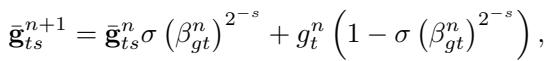
Comparing gradient averages over multiple windows gives the optimizer information about curvature and noise, improving stability and adaptability.
By comparing these, the RNN can estimate how noisy the gradient is and how the loss surface is evolving—critical clues for adjusting step sizes dynamically.
3. Dynamic Input Scaling
Borrowing ideas from RMSProp and ADAM, the optimizer rescales gradient magnitudes before feeding them into the RNN. This ensures stable behavior regardless of parameter scale.
Dynamic input scaling ensures gradients remain well-conditioned, improving training stability.
Additionally, it computes relative gradient magnitudes across parameters, helping the network understand how different parts of the model evolve.
Relative scaling lets the optimizer compare how gradient magnitudes change across layers and timescales.
4. Separating Step Size from Direction
Classic adaptive optimizers separate what direction to move from how far to move. The learned optimizer enforces this same decomposition:
\[ \Delta \theta_t^n = \exp(\eta_{\theta t}^n) \frac{\mathbf{d}_{\theta t}^n}{||\mathbf{d}_{\theta t}^n|| / N_t} \]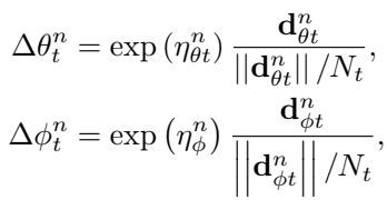
The optimizer decouples direction from step magnitude, improving robustness to parameter scaling.
Crucially, the RNN doesn’t output the learning rate directly—it predicts changes to the rate. This forces it to adapt dynamically across different tasks and timescales.
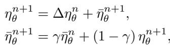
The learning rate evolves over time, helping the optimizer generalize across diverse problems.
Meta-Training: Teaching the Optimizer to Learn
A well-designed architecture needs an equally thoughtful training curriculum. Instead of training on large neural networks, the researchers built a compact but diverse set of synthetic optimization problems that capture the essence of real-world challenges.
A Diverse Training Ensemble
The meta-training set included:
- Classic pathological functions like Rosenbrock, Ackley, and Beale—difficult landscapes with sharp valleys and deceptive minima.
- Convex problems such as quadratic bowls and logistic regression tasks.
- Noisy gradient problems, including minibatched losses and stochastic noise injection.
- Slow-convergence tasks, where gradients are sparse or oscillatory.
- Transformed problems, applying variable scaling, power-law distortions, or multi-task mixups.
No neural networks were used. This diversity forced the optimizer to generalize loss-surface behaviors rather than memorizing neural-network-specific quirks.
The Meta-Objective: Focus on Precise Convergence
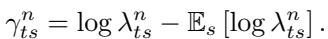
Instead of minimizing average loss, the authors minimized the logarithm of the loss at each step.
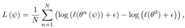
The log loss objective rewards optimizers that precisely drive function values toward zero, encouraging high-accuracy convergence.
This subtle tweak strongly rewards optimizers that push all the way to the minimum rather than stopping near it—teaching the learned optimizer fine-grained convergence control.
Training for Long Horizons
One of the core failures of previous learned optimizers was short-term bias: they were only trained for a few dozen steps. To address this, the authors drew the number of steps per training example from a heavy-tailed distribution, forcing the optimizer to handle both short and long training runs gracefully.
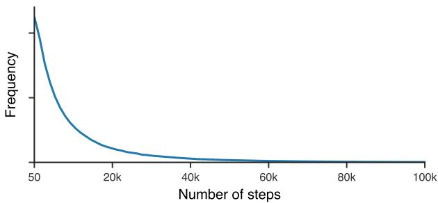
Long unrolls teach the optimizer to remain stable over thousands of iterations.
Experiments: Putting It to the Test
After meta-training, how does the learned optimizer perform in practice?
Home Turf: Meta-Training Tasks
On the synthetic problems used for training, it consistently matches or beats ADAM and RMSProp.

Figure 3. Learned optimizer performance exceeds traditional methods on the training corpus.
Generalization to New Architectures
The real triumph comes when applying the optimizer to unseen problems—such as training neural networks on the MNIST dataset. Despite never having seen a neural network during meta-training, the optimizer performs competitively with tuned standard methods.
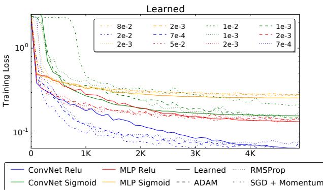
Figure 4a. The learned optimizer successfully trains both ConvNets and fully connected networks on MNIST.
Scaling Up to ImageNet
Astonishingly, the learned optimizer also handles full-scale deep models like InceptionV3 and ResNetV2 on ImageNet. For the first 10,000–20,000 iterations, its performance mirrors optimizers meticulously tuned for those architectures.

Figure 4b. Early optimization performance on ImageNet rivals state-of-the-art manual optimizers.
Though training eventually plateaus, the fact that a learned optimizer trained on toy problems can stably train ImageNet-scale models for thousands of steps is unprecedented.
Robustness to Learning Rate Initialization
Choosing learning rates is notoriously finicky. The learned optimizer, however, shows much greater robustness across a wide range of initial values.
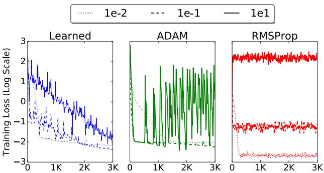
Figure 5. Learned optimizer generalizes across learning rate settings better than ADAM or RMSProp.
Ablation Studies: Why Every Feature Matters
Removing architectural components—like attention, multi-timescale momentum, or the logarithmic meta-objective—degrades performance significantly. Each piece contributes meaningfully to stability and convergence.
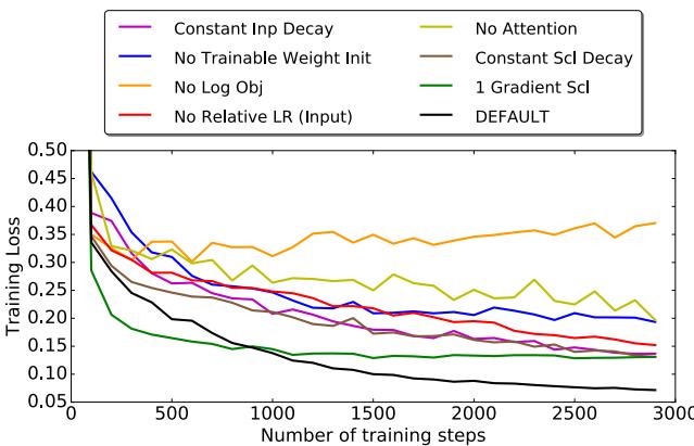
Figure 6. Every design choice strengthens generalization and performance.
Wall-Clock Comparison
While the learned optimizer incurs more overhead at small batch sizes, that gap narrows as batch size grows. Eventually, its runtime approaches that of standard optimizers.
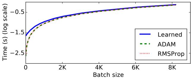
Figure 7. Runtime scalability improves with larger batches, making learned optimization practical for big models.
Conclusion: Learning to Learn at Scale
Wichrowska and colleagues achieved what was once thought impossible: a learned optimizer that generalizes to entirely new tasks and scales to massive architectures.
Their key ingredients—hierarchical RNN coordination, optimization-inspired features, and a diverse, long-horizon meta-training curriculum—together unlock powerful general-purpose learning behavior.
While challenges remain (such as sustaining progress in late training), this research transforms learned optimizers from a novelty into a credible successor to hand-tuned methods.
The broader implication is profound: if we can teach AI to optimize anything—even its own learning—we edge closer to systems that truly learn how to learn.
The next generation of optimizers may not be crafted by human intuition—but discovered by machines themselves.