Learning to Learn Fast: A Deep Dive into Meta-SGD

Introduction: The Thirst for Data

Modern deep learning is a marvel—but it’s also a glutton for data. Models such as large-scale vision and language systems thrive on huge datasets, sometimes requiring weeks of computation. This approach works when data is abundant, but what happens when it’s not? How do we train a system to identify rare animal species from just a few photos or help a robot learn to manipulate a new object after seeing it once?

This is the challenge of few-shot learning: enabling models to generalize from very limited data. Humans are naturally good at this—show a child a picture of a zebra, and they can recognize zebras again, even from one glimpse. Machine learning models, however, typically need thousands of examples. Bridging that gap is one of AI’s most fascinating frontiers.

The key idea lies in shifting from learning to learning to learn—a field known as meta-learning. Instead of training a model on a single massive dataset, we train a “meta-learner” across a variety of small, related tasks. The meta-learner discovers the principles of fast adaptation—how to learn new tasks efficiently from just a handful of samples.

This article explores one of the landmark studies in this area: “Meta-SGD: Learning to Learn Quickly for Few-Shot Learning.” The authors present a method that not only learns a good starting point for a model but also learns how to update that model. Meta-SGD learns its own version of Stochastic Gradient Descent (SGD)—tailored for rapid adaptation. Remarkably, it achieves state-of-the-art performance after just one update step.

Background: The Rise of Meta-Learning

Meta-learning operates across two interconnected loops, working on different timescales:

1. Inner Loop (Fast Learning): A “learner” model is trained on a small, specific task—for example, classifying five new flower species using just one image per class. This occurs quickly, often in a single or few updates.
2. Outer Loop (Slow Learning): The “meta-learner” watches these learners adapt and measures how well they generalize. It adjusts its own parameters to refine this process. Repeating this across a wide range of tasks gradually teaches the meta-learner the universal principles of learning itself.

Picture the inner loop as a student mastering a subject for a pop quiz; the outer loop is the teacher improving their teaching strategy after hundreds of quizzes.

Before Meta-SGD, researchers explored three types of meta-learning:

• Metric-based methods (e.g., Matching Networks, Siamese Networks): These learn an embedding space where distance metrics help classify new samples with few labels.
• Memory-based methods (e.g., Memory-Augmented Neural Networks, or MANNs): These rely on recurrent structures like LSTMs to store prior experiences for quick retrieval.
• Optimization-based methods: These directly learn how to train models—the focus of Meta-SGD. The well-known MAML (Model-Agnostic Meta-Learning) learns an initialization of weights \( \theta \) that allows quick adaptation using standard SGD on new tasks.

However, MAML learns only the initialization \( \theta \). The learning rate and how updates should occur remain manually tuned. The authors of Meta-SGD asked: what if we could learn the optimization process itself?

The Core Method: Supercharging Gradient Descent

Classic Stochastic Gradient Descent (SGD) updates parameters \( \boldsymbol{\theta} \) using the rule:

\[ \boldsymbol{\theta}^{t} = \boldsymbol{\theta}^{t-1} - \alpha \nabla \mathcal{L}_{\mathcal{T}}\left(\boldsymbol{\theta}^{t-1}\right) \]

This has three key components, traditionally hand-engineered:

1. Initialization (\( \boldsymbol{\theta}^{0} \)) – usually random.
2. Update Direction (\( \nabla \mathcal{L_{\mathcal{T}}} \)) – the negative gradient, i.e., steepest descent.
3. Learning Rate (\( \alpha \)) – a scalar determining step size.

MAML meta-learns only the initialization \( \boldsymbol{\theta} \). Meta-SGD takes it further: it learns all three ingredients—initialization, direction, and learning rate.

The core update rule of Meta-SGD: each parameter has its own learned learning rate and direction modifier.

Here’s the intuition:

• \( \boldsymbol{\theta} \): Meta-learned initialization—a strong starting point for new tasks.
• \( \nabla \mathcal{L}_{\mathcal{T}}(\boldsymbol{\theta}) \): Gradient on the training samples for a given task.
• \( \boldsymbol{\alpha} \): A vector of the same dimension as \( \boldsymbol{\theta} \), learned during meta-training, encoding both per-parameter learning rate and sign.
• \( \circ \): Element-wise multiplication.

By making the learning rate a vector, Meta-SGD achieves two powerful effects:

1. Per-Parameter Learning Rates: Each weight learns its own optimal step size.
2. Learned Update Directions: Individual entries of \( \boldsymbol{\alpha} \) can be negative, altering the direction of updates relative to standard gradients.

This means Meta-SGD can steer optimization toward better generalization rather than pure loss minimization. It essentially redefines the trajectory of learning through experience—an optimizer that learns how to optimize.

Meta-learning happens slowly across tasks (black line), while rapid adaptation occurs within tasks (red arrows). Meta-SGD learns both initialization and update strategy.

The Meta-Training Loop

During meta-training, the model learns both initialization \( \boldsymbol{\theta} \) and adaptation parameters \( \boldsymbol{\alpha} \) by minimizing the expected test loss after inner-loop updates.

The objective minimizes the expected loss on test sets after task-specific adaptation.

Concretely:

1. Sample a batch of tasks \( \mathcal{T}_i \sim p(\mathcal{T}) \), each with a train and test split.
2. Inner Loop: For each task, compute gradient \( \nabla \mathcal{L}_{\text{train}(\mathcal{T}_i)}(\boldsymbol{\theta}) \), then adapt using \[ \boldsymbol{\theta}_i' = \boldsymbol{\theta} - \boldsymbol{\alpha} \circ \nabla \mathcal{L}_{\text{train}(\mathcal{T}_i)}(\boldsymbol{\theta}) \]
3. Evaluate on Test Set: Compute \( \mathcal{L}_{\text{test}(\mathcal{T}_i)}(\boldsymbol{\theta}_i') \) to gauge generalization.
4. Outer Loop: Update \( (\boldsymbol{\theta}, \boldsymbol{\alpha}) \) via gradient descent on accumulated test losses.

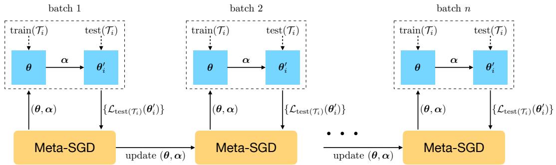
During training, batches of tasks teach the meta-learner how to initialize and adapt optimally.

Algorithm 1 summarizes the process for supervised learning tasks.

The same principle applies to reinforcement learning—where tasks are entire Markov Decision Processes (MDPs) and the loss is the negative expected return. Meta-SGD learns an initial policy and its adaptation rule for new environments.

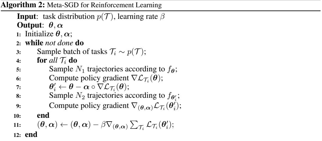
Algorithm 2 outlines Meta-SGD applied to reinforcement learning via policy gradient updates.

Experiments & Results: Putting Meta-SGD to the Test

The authors tested Meta-SGD in three domains—regression, classification, and reinforcement learning—and compared it to strong baselines like MAML.

Few-Shot Regression

The first experiment tackled K-shot regression: fitting a sine wave given only K data points.

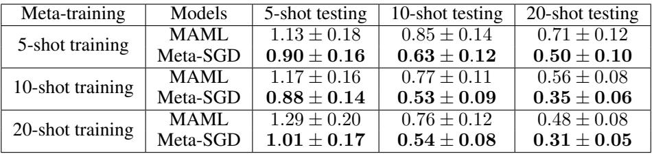
Table 1: Meta-SGD consistently achieves lower Mean Squared Error than MAML, indicating better adaptation.

Meta-SGD’s advantage is clear—it outperforms MAML across all configurations. By meta-learning both initialization and update strategy, it learns an optimization path that better captures underlying structure.

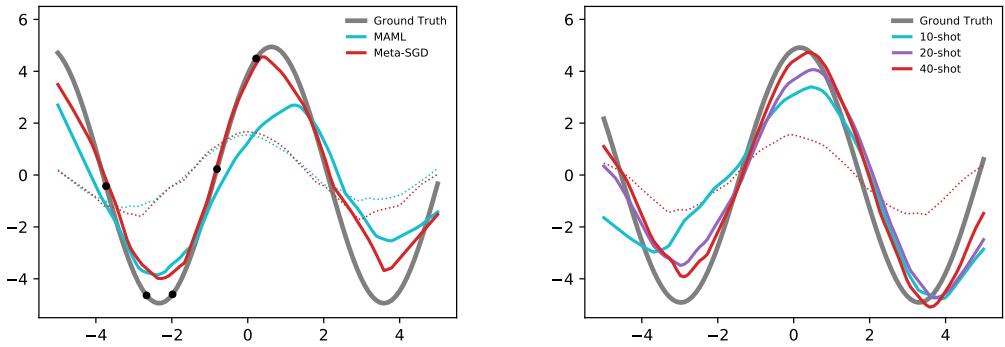
Figure 3: Meta-SGD adapts more effectively with limited data. The red curve aligns closely with the true sine wave after only one update.

In the 5-shot example (left panel), where all samples lie on one side of the curve, MAML struggles to generalize, while Meta-SGD seamlessly learns the full sinusoidal shape. The learned optimizer clearly adapts in a more generalizable direction.

Few-Shot Classification

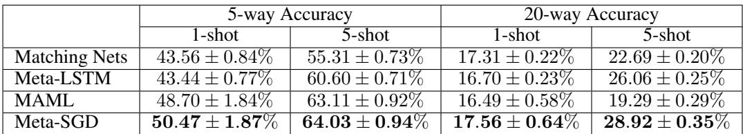
Meta-SGD was evaluated on two key benchmarks—Omniglot and MiniImagenet.

Omniglot, a database of handwritten characters, tests one-shot and few-shot recognition:

Meta-SGD slightly exceeds other models, reaching near-perfect results on Omniglot few-shot classification.

MiniImagenet expands the challenge to real-world images:

Meta-SGD provides substantial gains on MiniImagenet, significantly outperforming other approaches.

Across both datasets, Meta-SGD reaches or surpasses prior state-of-the-art accuracy—trained with only one-step adaptation. This makes it extraordinarily efficient for new tasks without sacrificing performance.

Few-Shot Reinforcement Learning

In the reinforcement learning domain, Meta-SGD was tested on a 2D navigation task where an agent must move from a start position to a goal.

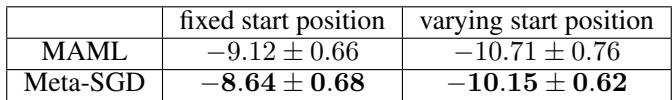
Table 4: Meta-SGD leads to higher average returns in 2D navigation tasks compared with MAML.

Agents trained via Meta-SGD adapt faster and achieve higher rewards. Visualizing their trajectories reveals why:

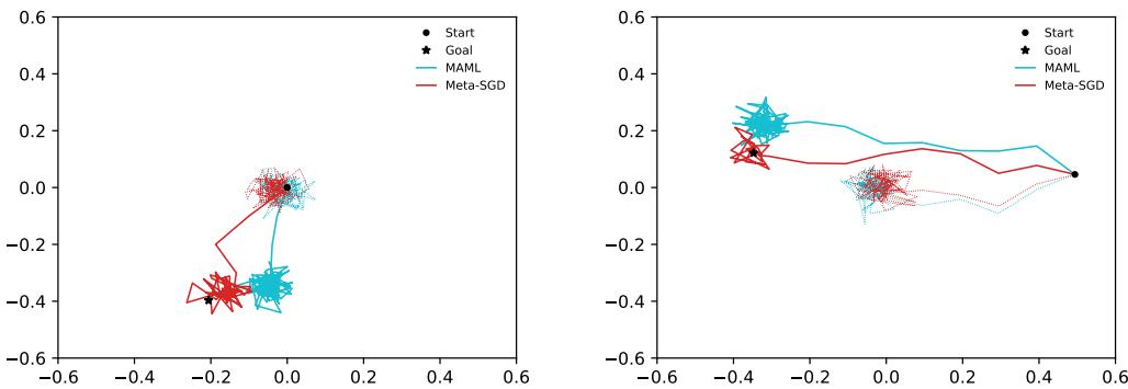
Figure 4: Meta-SGD produces smoother, more direct paths to the goal. Its policy updates are more efficient and confident.

These results show that Meta-SGD’s learned update rules outperform traditional gradient-based adaptation, even when applied to dynamic learning environments.

Conclusion & Implications

The Meta-SGD study introduces a paradigm shift: instead of manually designing optimizers, we can learn them. By meta-learning initialization, direction, and per-parameter learning rates, Meta-SGD creates a customized optimization procedure that adapts rapidly and effectively across tasks.

Key Takeaways:

• Higher Capacity: Meta-SGD learns every component of the optimization process, surpassing MAML’s single initialization meta-learning.
• Rapid Adaptation: It achieves top results after just one step, enabling fast, on-the-fly learning.
• Versatility: It works remarkably well across regression, classification, and reinforcement learning domains.

Meta-SGD paves the path toward more autonomous learning systems—optimizers that evolve through experience rather than human tuning. Future exploration could address scaling Meta-SGD to large models and cross-domain transitions, enabling models that truly learn to learn in the spirit of human cognition.