](https://deep-paper.org/en/paper/1803.00676/images/cover.png)
Humans have a remarkable ability to learn new concepts from just one or two examples. See a single photo of a platypus, and you can likely identify another one—even if it’s from a different angle. Modern AI, particularly deep learning, struggles with this. While these models can achieve superhuman performance in tasks like image recognition, they typically require massive datasets with thousands of labeled examples for every category. This gap between human and machine learning is a major hurdle in our quest to build flexible and adaptable AI systems.
The field of few-shot learning aims to close this gap by designing models that can generalize from a handful of labeled examples. A popular approach is meta-learning, or learning to learn, where a model trains on a wide variety of small learning tasks to develop a general strategy for adaptation. Yet most few-shot research assumes that all available data are labeled. What if, in addition to a few labeled examples, we also have a large pool of unlabeled data? This scenario is not only more realistic—it’s closer to how humans learn in messy, unlabeled environments.
A 2018 paper from researchers at the University of Toronto, Google Brain, and MIT explores this question. In “Meta-Learning for Semi-Supervised Few-Shot Classification,” the authors extend the few-shot learning paradigm to a more practical, semi-supervised setting. They show how models can leverage unlabeled data—including irrelevant “distractor” images—to improve predictions dramatically. This work marks a key step toward building AI that learns with minimal supervision, much like we do.
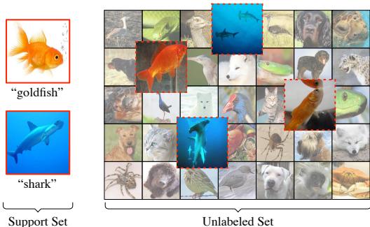
Figure 1: Semi-supervised few-shot setup. The learner has labeled samples of two fish species and a large pool of unlabeled sea life, including irrelevant distractors.
Background: Learning to Learn with Prototypical Networks
To understand the contribution of this research, we first need to recall the foundations of few-shot learning and one of its most influential models—Prototypical Networks.
The Episodic Training Paradigm
Modern few-shot learning typically uses episodic training, which simulates the few-shot scenario repeatedly during meta-training. Instead of training on the entire dataset at once, the model is presented with many small episodes, each representing a miniature classification task.
Each episode contains:
- A Support Set (S): A small labeled training set containing
Kexamples of each ofNclasses. - A Query Set (Q): A set of unlabeled examples from the same
Nclasses, used for evaluation within the episode.
The model learns to classify the query examples based on the labeled support examples. Losses are computed from its predictions on the query set, and model parameters are updated accordingly. Training on numerous randomized episodes teaches the system how to build effective small-sample classifiers—essentially, how to learn to learn.
Prototypical Networks (ProtoNets)
Introduced by Snell et al. (2017), Prototypical Networks provide a clean and effective method for few-shot classification. Their key insight is to embed inputs into a feature space where examples from the same class are close together.
Embedding: A neural network maps each input image \(x\) to a vector \(h(x)\) in an embedding space, clustering similar classes together.
Prototype Calculation: For each class \(c\) in the support set, the network computes a prototype vector—the mean of the embeddings for that class.
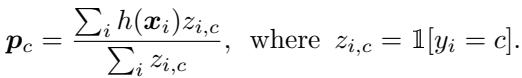
Equation 1: Prototype computation based on class-wise averages of embeddings.
- Classification: To classify a new query example \(x^*\), the model embeds it with \(h(x^*)\) and computes its distance to every class prototype. The probability that \(x^*\) belongs to class \(c\) is obtained via a softmax over the negative distances—whichever prototype is closest usually wins.
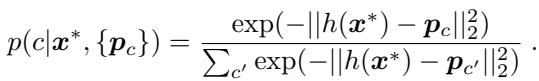
Equation 2: Query classification based on distances to prototypes.
The loss over an episode is the average negative log-probability of the correct prediction:
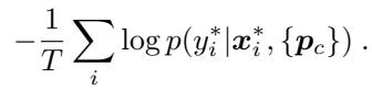
Equation 3: Optimization objective for training Prototypical Networks.
ProtoNets are elegant in their simplicity—they learn a good metric space where class clusters can be easily formed and compared.
Semi-Supervised Few-Shot Learning
The authors extend this episodic framework by adding a third component to each episode: an unlabeled set \(\mathcal{R}\), containing examples with no labels.
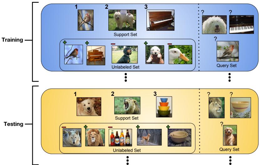
Figure 2: Semi-supervised training and testing episodes include unlabeled examples from relevant and distractor classes.
The challenge is to make use of these unlabeled examples—some likely belong to the same classes as the support samples, while others are distractors. The authors’ solution: use unlabeled data to refine the prototypes initially computed from the labeled support set. These improved prototypes yield better generalization to query data.
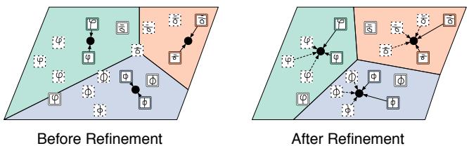
Figure 3: Prototype refinement using unlabeled examples.
The paper proposes three progressively advanced refinement strategies.
1. Refining Prototypes with Soft k-Means
The simplest idea borrows from soft k-means clustering. Prototypes act as cluster centers, and the unlabeled points are softly assigned to these clusters. Each prototype is then updated to better represent all examples—both labeled and unlabeled—of its class.
Process overview:
- Initialize prototypes from labeled support examples.
- Compute soft assignments: Each unlabeled point gets a probabilistic membership value for every class, based on its distance to the prototypes.
- Refine: Update the prototypes using a weighted average that includes labeled samples (hard assignments) and unlabeled examples (soft assignments).

Equation 4: Refinement via soft k-means.
Empirically, one refinement step proved sufficient to boost performance significantly.
2. Handling Distractors with an Extra Cluster
Soft k-means assumes that every unlabeled example belongs to one of the \(N\) known classes. In real scenarios, that’s rarely true—many unlabeled examples may be distractors. They can corrupt prototypes by pulling them toward irrelevant regions.
To guard against this, the authors introduce an extra distractor cluster. This \((N+1)\)th cluster captures unlabeled items that don’t fit any of the task’s classes, absorbing outliers and preventing them from misguiding the real class prototypes.
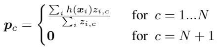
Equation 5: Adding a distractor cluster to handle unrelated examples.
Cluster-specific length-scales (\(r_c\)) allow the distractor cluster to spread more broadly, accommodating diverse outliers without disturbing the main structure.
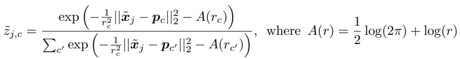
Equation 6: Soft assignment modified for distractor robustness.
3. A More Sophisticated Approach: Masked Soft k-Means
The final and most advanced extension, Masked Soft k-Means, learns to selectively ignore distractors. Instead of lumping all outliers into one cluster, the network learns a mask that determines how much each unlabeled example should influence each prototype.
The method unfolds as follows:
- Normalize Distances: For each unlabeled sample–prototype pair, compute a normalized distance \( \tilde{d}_{j,c} \).
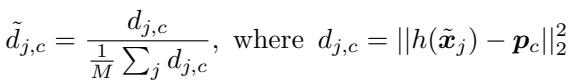
Equation 7: Normalized distances used for adaptive masking.
- Predict Mask Parameters: A small MLP analyzes statistics (e.g., min, max, variance, skew, kurtosis) of these distances and predicts threshold \(\beta_c\) and slope \(\gamma_c\) values per class.

Equation 8: Learning adaptive masking parameters.
- Compute Masks and Refine: Each unlabeled example receives a mask value \(m_{j,c}\) via a sigmoid function. If it’s close to the prototype (below threshold), the mask is near 1; otherwise, near 0. These masks weight the example’s influence when computing new prototypes.

Equation 9: Prototype refinement with learned masks to exclude distractors.
Because everything is differentiable, the MLP and refinement process are trained jointly. The model thus learns not just an embedding space—but a principled method for filtering irrelevant unlabeled data.
Experiments and Results
To test their framework, the authors evaluated on three datasets:
- Omniglot: Handwritten characters from 50 alphabets.
- miniImageNet: A reduced version of ImageNet, often used for few-shot benchmarks.
- tieredImageNet: A larger, hierarchically organized subset introduced in this paper, ensuring distinct training and testing categories.
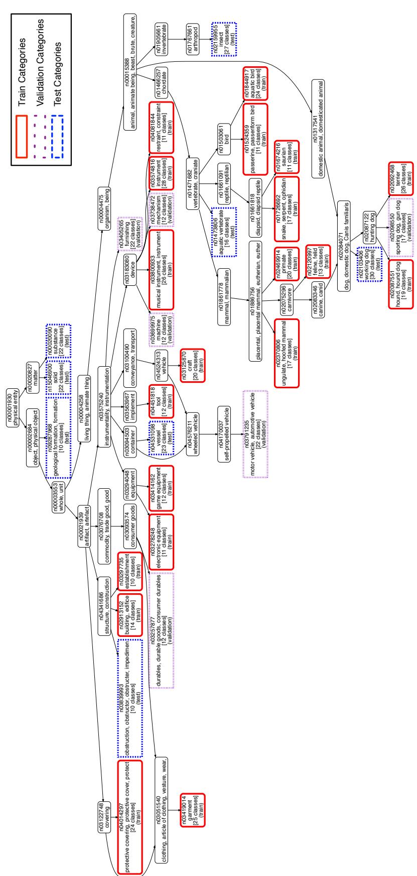
Figure 5: The hierarchical category split of tieredImageNet enforces meaningful dissimilarity between train and test classes.
Baseline comparisons:
- Supervised: Standard Prototypical Network ignoring unlabeled data.
- Semi-Supervised Inference: A supervised ProtoNet refined during testing with one k-means step.
Across all datasets, the semi-supervised variants dramatically improved performance.
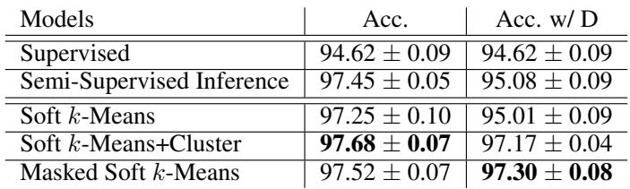
Table 1: Omniglot results show strong gains from semi-supervised refinement.
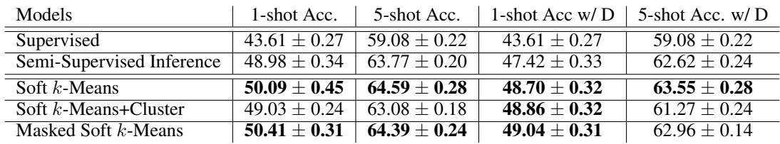
Table 2: Semi-supervised approaches outperform baselines on miniImageNet.
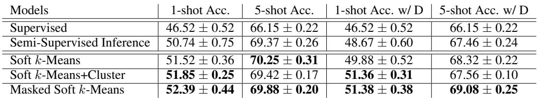
Table 3: TieredImageNet results confirm the advantage of using unlabeled data even with distractors.
Key Observations:
- Unlabeled Data Helps: All semi-supervised models outperform the supervised baseline—clear proof that unlabeled samples strengthen few-shot learning.
- Meta-Training Matters: Models trained end-to-end for refinement outperform inference-only variants, showing that learning to refine prototypes is itself beneficial.
- Masked k-Means Excels with Distractors: The masking model handles unseen classes gracefully, performing nearly as well in noisy conditions as in clean settings.
Performance also rose steadily as more unlabeled examples were available at test time—even beyond training conditions—demonstrating robust generalization.
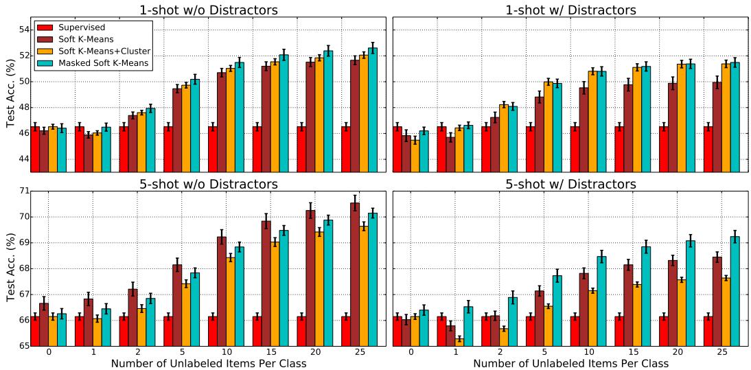
Figure 4: Accuracy improves consistently with more unlabeled items per class.
Finally, examining the learned masks revealed a bimodal distribution: mask values cluster near 0 or 1, indicating the model confidently distinguishes useful from irrelevant samples.
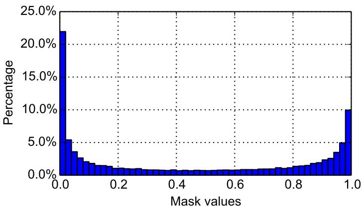
Figure 7: Mask distributions learned for Omniglot, showing decisive inclusion–exclusion behavior.
Conclusion and Implications
This research takes few-shot learning into a more realistic semi-supervised realm, bridging the gap between meta-learning, semi-supervised learning, and clustering. The findings show that unlabeled data—even noisy, imperfect data—can meaningfully improve model accuracy when integrated intelligently.
The key takeaways:
- A new learning framework: The first formal definition and benchmark adaptation for semi-supervised few-shot learning.
- Refined models: Three extensions to Prototypical Networks that use unlabeled data efficiently, with Masked Soft k-Means emerging as the most robust.
- A stronger benchmark: The tieredImageNet dataset introduces structure that better reflects real-world conditions.
By learning how to benefit from unlabeled samples within each task, these models exhibit human-like adaptability. In a world overflowing with data but sparse labels, such approaches pave the way for smarter, more efficient AI—capable of thriving even when supervision is scarce.