](https://deep-paper.org/en/paper/2209.00796/images/cover.png)
From hyper‑realistic portraits of people who don’t exist to epic landscapes painted from a single sentence, diffusion models power many of today’s most impressive generative systems. In a short span of years, they have gone from a promising theory to the backbone of state‑of‑the‑art systems for image, video, 3D, audio, and even molecular design.
This article is a guided tour of the survey “Diffusion Models: A Comprehensive Survey of Methods and Applications” (Yang et al., 2023). My aim is to take you from the core intuition to the technical foundations, then through the major research directions and the most exciting applications. Wherever helpful, I’ll use figures from the paper to illustrate the ideas.
If you’re a student or practitioner trying to make sense of the literature, consider this a compass: the map, the major routes people take on it, and the notable landmarks.
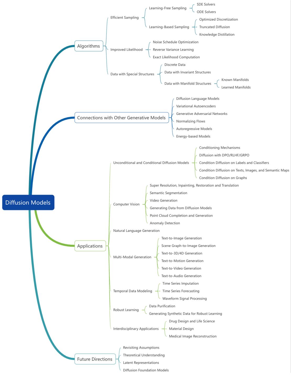
Fig. 1 — High-level taxonomy of diffusion‑model research covered in the survey: core algorithmic variants, efficient sampling methods, likelihood improvements, domain adaptations, connections to other generative families, applications, and future directions.
Table of contents
- Foundations — the two simple ideas behind powerful models
- Three mathematical views: DDPM, score matching, and SDEs
- Making diffusion fast: sampling methods
- Tightening likelihoods and principled training
- Adapting diffusion to non-image domains and structures
- How diffusion connects to VAEs, GANs, flows, autoregressive and energy models — and LLMs
- Applications: vision, multi‑modal, audio, time series, molecules, and medicine
- What’s next: promising research directions
- Wrap up
Foundations — destruction + reconstruction
At its heart, a diffusion model implements two processes:
- A fixed, forward process that gradually corrupts (adds noise to) real data until it becomes a simple tractable distribution (usually Gaussian noise).
- A learnable reverse process that starts from noise and gradually denoises back to a data sample.
This “destruction then reconstruction” strategy turns density estimation into a sequence of local denoising problems. Intuitively, each denoising step only needs to make a small, local correction — a task neural networks can learn reliably.
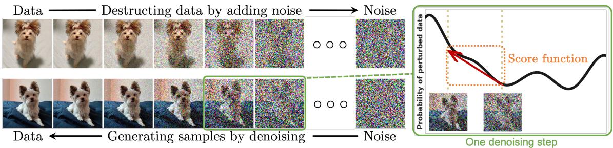
Fig. 2 — The forward process slowly injects Gaussian noise into a clean example until it looks like noise; the trained reverse process removes that noise step by step to generate new samples. The right panel visualizes the score direction: at each noisy level, the score points toward regions of higher data density.
We will now make those ideas precise through three dominant formalisms used in the literature.
Three mathematical views that are equivalent in spirit
The survey frames diffusion models through three complementary lenses. Each brings intuition and practical algorithms.
1) Denoising diffusion probabilistic models (DDPMs)
DDPMs set up two discrete Markov chains:
- Forward chain q(x_t | x_{t-1}) — a simple, fixed sequence of Gaussian corruption steps that eventually turns data into near‑Gaussian noise.
- Reverse chain p_theta(x_{t-1} | x_t) — learned; a neural network parameterizes the mean and (optionally) the variance of each reverse kernel.
A common forward kernel is
\[ q(x_t \mid x_{t-1}) = \mathcal{N}\big(x_t; \sqrt{1-\beta_t}\,x_{t-1},\; \beta_t I\big), \]where the schedule \(\{\beta_t\}\) controls the noise added at each step. A useful property of this choice is that you can sample \(x_t\) at any time \(t\) directly from \(x_0\):
\[ x_t = \sqrt{\bar\alpha_t}\,x_0 + \sqrt{1-\bar\alpha_t}\,\epsilon,\quad \epsilon\sim\mathcal{N}(0,I), \]with \(\bar\alpha_t=\prod_{s=1}^t (1-\beta_s)\).
Training maximizes a variational lower bound (VLB) on data log‑likelihood. Ho et al. popularized a reparametrization that leads to a simple and effective training objective: predict the injected noise \(\epsilon\) from \(x_t\) and \(t\). The resulting loss is
\[ \mathbb{E}_{t,x_0,\epsilon}\big[\lambda(t)\,\|\epsilon - \epsilon_\theta(x_t,t)\|^2\big], \]which is numerically stable and empirically effective.
Remarks:
- DDPMs are conceptually simple and easy to implement.
- Sampling is iterative and often requires many network evaluations (hundreds to thousands of steps), which motivates later research on faster samplers.
2) Score‑based generative models (SGMs)
Score models approach the problem by learning the score function of noisy data distributions:
\[ s_\theta(x,t)\approx\nabla_x\log q_t(x), \]where \(q_t\) is the density of \(x_t\) after adding Gaussian noise with variance \(\sigma_t^2\). Once you have score estimates at a sequence of noise levels, you can sample by Langevin dynamics or other score‑based samplers: take small steps in the direction of the score and add a bit of Gaussian noise to encourage exploration.
The training objective is a multi‑scale denoising score matching loss, which, after algebraic manipulation, is equivalent to the DDPM loss under appropriate parameterizations. This equivalence is central: DDPM and SGMs are different views on the same underlying denoising task.
3) Continuous limit: Score SDEs and the probability flow ODE
Both DDPMs and SGMs can be seen as discretizations of a continuous‑time stochastic differential equation (SDE)
\[ d x = f(x,t)\,dt + g(t)\,d w_t, \]with \(w_t\) Brownian motion. The forward diffusion is an SDE that blurs data into noise. Anderson’s theorem gives the form of the reverse‑time SDE; critically, the reverse drift includes the score \(\nabla_x\log q_t(x)\). If we can estimate that score, we can solve the reverse SDE to generate samples.
There is also a deterministic ODE — the probability flow ODE — whose trajectories have the same marginal distributions as the SDE. Solving the ODE yields deterministic sampling schemes and gives a direct link to continuous normalizing flows, enabling exact (or tightly bounded) evaluation of log densities at the cost of solving ODEs.
Why these views matter:
- DDPMs are convenient and easy to train.
- SGMs give intuition about the score field and allow MCMC samplers.
- Score SDEs and the probability flow ODE unify these perspectives and unlock methods for likelihood evaluation and alternative deterministic samplers.
Fast sampling: making diffusion practical
The biggest practical complaint about diffusion models is sampling cost. Early models needed hundreds or thousands of sequential denoising steps. The survey organizes progress on this problem into two families: learning‑free numerical solvers, and learning‑based approaches (distillation, optimized discretizations, etc.).
Learning‑free solvers: smarter discretizations
These methods keep the pre‑trained model and focus on better numerical methods for the reverse SDE or the probability flow ODE.
- ODE solvers: DDIM introduced deterministic samplers that correspond to special discretizations of the probability flow ODE; many later methods (Heun’s method, DPM‑Solver, diffusion exponential integrators) exploit higher‑order numerical integration schemes or the semi‑linear structure of the ODE to drastically reduce the required steps (often to 10–50) with preserved sample quality.
- SDE solvers & predictor–corrector: Stochastic samplers can give better mixing or fidelity. Predictor–corrector schemes pair a coarse SDE or ODE step (predictor) with score‑guided MCMC refinement (corrector). Adaptive step‑size control and Langevin “churn” steps have also improved efficiency while keeping quality high.
Key tradeoff: deterministic ODE solvers are often faster (fewer evaluations) but can degrade diversity or fidelity slightly; stochastic solvers can be higher quality but typically require more steps.
Learning‑based accelerations
These methods train additional components to speed sampling.
- Knowledge distillation: Progressive distillation trains a fast “student” sampler to mimic the multi‑step teacher; repeating the procedure can halve the steps at each distillation stage.
- Optimized discretization: Given a trained model, one can search for an optimal small set of time points (discretization schedule) to maximize sample quality. Differentiable search techniques and dynamic programming have been applied here.
- Truncated diffusion: Stop the forward noising early and start reverse generation from a non‑Gaussian (but structured) distribution modeled by a faster generator (e.g., a VAE or GAN). This shortens the diffusion path but requires integrating another model.
Practical impact: With these techniques, modern systems routinely generate high‑quality images in 10–50 network calls — sometimes approaching real‑time performance under the right engineering budget.
Improving likelihood: from heuristics to principled objectives
Diffusion training often targets a VLB, but that bound can be loose. The survey groups likelihood improvement efforts into three directions.
Noise schedule optimization: The choice of \(\beta_t\) (or continuous analogues) matters for both sample quality and likelihood. Works like iDDPM and Variational Diffusion Models (VDMs) learn optimal continuous schedules, sometimes parameterized with monotone neural networks, to tighten the VLB.
Reverse variance learning: Early DDPMs used fixed reverse variances; learning the reverse variance or deriving optimal analytic forms from score estimates (Analytic‑DPM) improves the VLB and provides better likelihood estimates.
Exact likelihood / ScoreFlows: In the continuous SDE view, one can derive bounds and variational objectives that directly target the likelihood of samples generated by the reverse SDE or the probability flow ODE. ScoreFlows and related approaches exploit that connection, enabling principled maximum likelihood training and tighter log‑density estimation (albeit at higher computational cost due to trace/ODE estimations).
Why this matters: tighter likelihoods strengthen diffusion models as proper probabilistic models (not only samplers). For applications requiring calibrated densities (anomaly detection, some scientific tasks), these advances are crucial.
Adapting diffusion to structured and non‑standard data
The canonical diffusion setup assumes continuous Euclidean data with Gaussian corruption. Many data domains violate that. The survey presents methods to extend diffusion to:
Discrete data (text, categorical tokens)
Gaussian noise is inappropriate for discrete spaces. Solutions include:
- Random walk or masking corruption processes on discrete state spaces (e.g., multinomial diffusion, absorbing states).
- Concrete score matching: finite‑difference analogues of score matching for discrete variables.
- Continuous time Markov chain formalisms that generalize discrete diffusion to continuous time, enabling efficient samplers.
These methods have enabled diffusion‑style generation for text, symbolic sequences, and discrete symbolic modalities.
Data with symmetry / invariance (graphs, point clouds, molecules)
Many datasets obey symmetries (permutation invariance for graphs, rotational/translation invariance for 3D molecules). To respect these, models must be equivariant:
- Use permutation‑equivariant GNNs for graphs so that the learned reverse kernels preserve permutation invariance of generated graphs.
- For 3D molecular coordinates, build equivariant score networks (E(3) / SE(3) equivariance) so denoising commutes with rotations/translations. This preserves physical properties (e.g., energy invariances) and improves sample quality.
Data on manifolds (spherical climate data, constrained domains)
If data lives on a known manifold, one can:
- Formulate SDEs on Riemannian manifolds and adapt score matching to the manifold geometry.
- Use extrinsic or intrinsic constructions (Riemannian score models, geodesic random walks) to perform diffusion directly on the manifold.
When the manifold is unknown, latent diffusion is a popular practical alternative: learn an encoder (autoencoder / VAE) that maps data to a lower‑dimensional latent manifold, then run diffusion in that latent space (Latent Diffusion Models, LDMs). Latent approaches make training and sampling cheaper and are the basis for large systems like Stable Diffusion.
Diffusion and other generative families — complementary strengths
Diffusion models don’t replace other generative paradigms; they complement them. The survey lays out several important connections.
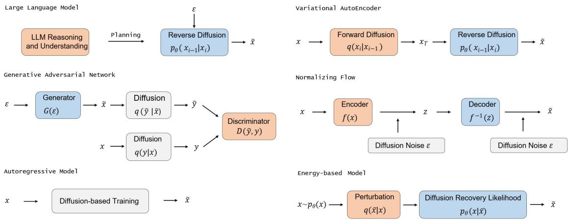
Fig. 3 — How diffusion components plug into different generative architectures: LLMs can act as planners or controllers for region‑wise diffusion; VAEs provide latent spaces for efficient diffusion (LDMs); GANs can model denoising steps or stabilize training; flows and CNFs relate through the probability flow ODE; autoregressive and energy models share theoretical links to score matching.
Highlights:
- VAEs: DDPMs are closely related to infinitely deep hierarchical VAEs; combining autoencoders and diffusion (latent diffusion) yields large efficiency gains.
- GANs: Can be used to model denoising steps for larger transitions (fewer steps), or diffusion can regularize GAN training. Hybrid diffusion–GANs attempt to combine sample fidelity with fast synthesis.
- Normalizing flows / CNFs: The probability flow ODE connects diffusion to continuous flows; diffusion provides a robust way to model complex distributions without strict bijectivity constraints.
- Autoregressive models: Some diffusion formulations approximate autoregressive factorization; there are hybrid autoregressive diffusion models that trade off parallelizability and density estimation.
- Energy‑based models (EBMs): Score matching and EBMs are closely related — diffusion recovery likelihood provides a tractable way to train EBM sequences using diffusion reverse conditional distributions.
- LLMs: The most recent and exciting interactions pair the world‑knowledge and planning power of large language models with diffusion samplers for visual generation and editing. LLMs can parse complex prompts, plan compositions, and provide structural guidance enabling better compositional generation.
These cross‑fertilizations have led to practical systems that are more controllable, compositional, and capable.
Applications — where diffusion really shines
Diffusion models have been applied across many domains. I’ll highlight the most impactful applications and give a few representative examples.
Computer vision: generation, restoration, editing
- High‑fidelity unconditional and conditional image synthesis (DDPMs, LDMs): Imagen, GLIDE, Stable Diffusion, and related systems use conditional diffusion with text or other inputs to produce stunning images.
- Super‑resolution, inpainting, restoration: SR3, RePaint, DDRM, Palette, ConPreDiff — these models cast restoration as conditional denoising and achieve high perceptual quality.
- Semantic segmentation and representation learning: diffusion pretraining yields features useful for label‑efficient segmentation.
- Video generation: spatio‑temporal diffusion architectures and cascaded models produce short videos and are rapidly improving temporal consistency.
Figure: ConPreDiff inpainting example and editing datasets generated by EditWorld (two representative images).

Fig. 4 — Example inpainting results produced by ConPreDiff. Conditioning on partial inputs and context yields high‑quality reconstructions.
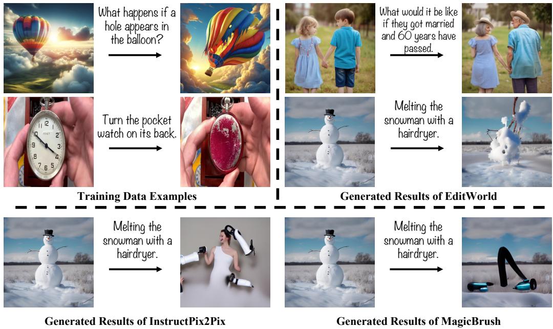
Fig. 5 — EditWorld synthesizes large, instruction‑following editing datasets that improve downstream editing models.
Multi‑modal: text→image, text→video, text→3D, and beyond
- Text‑to‑image: Stable Diffusion, DALLE‑2 (unCLIP), Imagen, and many later models use diffusion conditioned on text embeddings (CLIP/T5) with classifier‑free guidance, cross‑attention, and layout control.
- Compositional and controllable generation: Methods that use LLMs as planners (RPG, IterComp) break down complex prompts into regions or subprompts and improve compositionality.
- Text‑to‑video: Cascaded and factorized diffusion models (Imagen Video, Make‑A‑Video) extend image priors to temporal sequences.
- Text‑to‑3D and 3D asset generation: DreamFusion, Magic3D, and followups use 2D diffusion priors to optimize 3D representations (NeRFs, implicit functions).
- Audio and speech: WaveGrad, DiffWave, Grad‑TTS use score models and diffusion decoders for waveform synthesis and TTS.
Representative illustration: cross‑model comparisons for text‑to‑image.
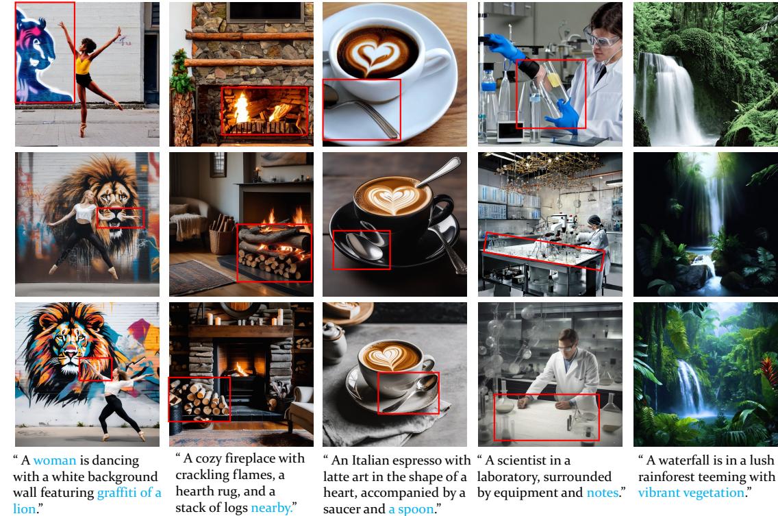
Fig. 6 — Qualitative comparison of text‑to‑image outputs from different diffusion backbones showing how conditioning and contextual modeling affect fidelity and alignment.
Time‑series and waveform modeling
- Imputation and forecasting: CSDI, SSSD and retrieval‑augmented diffusion methods (RATD) use conditional score models to provide principled uncertainty and data‑consistent imputations.
- Waveform generation: WaveGrad and DiffWave demonstrate high‑quality audio synthesis, trading steps for fidelity.
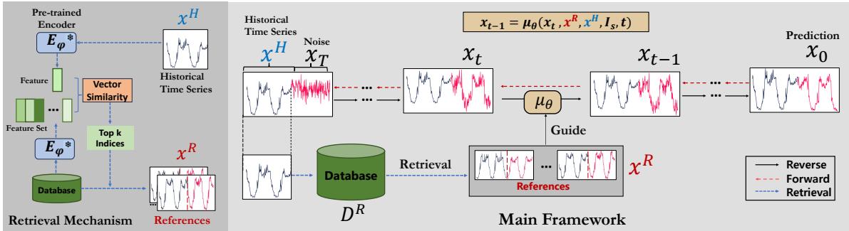
Fig. 7 — Retrieval‑augmented diffusion for time‑series forecasting: retrieve similar historical contexts and condition the denoising process for better forecasts.
Scientific and interdisciplinary applications
- Molecular and protein design: GeoDiff, Torsional Diffusion, ConfGF, and IPDiff generate molecular conformations and target‑aware ligands with equivariant models and protein‑conditioned priors.
- Materials and crystals: CDVAE and similar models generate periodic crystal structures.
- Medical imaging: Score‑based reconstruction methods solve inverse problems (MRI, CT) by uniting learned priors with measurement forward models.
Illustration: schematic from IRDiff/IPDiff showing protein‑conditioned ligand generation.
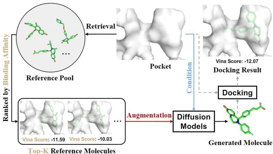
Fig. 8 — Retrieval‑augmented and interaction‑aware diffusion for structure‑based drug design: retrieval provides reference binding motifs; the diffusion model generates candidate ligands that are then evaluated by docking.
Practical guidance — when to use diffusion models
- Use diffusion when you need high‑quality, high‑diversity samples and robustness in training (they are more stable than GANs).
- Prefer latent diffusion (LDMs) when compute/memory is constrained: train the heavy workhorse in a compressed latent space.
- If you need fast sampling in production, invest in distillation or DPM‑Solver / exponential integrators; 10–20 steps are often achievable.
- For structured data (graphs, molecules, point clouds), choose equivariant architectures and domain‑aware corruption processes.
- If calibrated likelihoods matter, consider ScoreFlows or likelihood‑aware training objectives.
Open problems and future directions
The survey highlights important and exciting open directions:
- Revisiting assumptions: Can we design finite‑time bridges (Schrödinger bridge, optimal transport) that are more efficient than naive long diffusions?
- Theoretical understanding: Why do diffusion models generate such high‑quality samples? What are the optimal design choices for schedulers, parameterizations, and architectures?
- Latent and compact representations: How do we get diffusion models to learn meaningful, low‑dimensional latents that are useful for downstream tasks?
- Foundation models and AIGC: Can diffusion scale as a foundation technology the way LLMs did? Combining LLMs and diffusion is already fruitful — but what happens at scale across multi‑modal, multi‑task regimes?
- Efficiency vs fidelity tradeoffs: Achieving extremely fast sampling without sacrificing quality remains an engineering and theoretical frontier.
Closing thoughts
Diffusion models blend elegant theory with practical success. The core idea — learn to denoise progressively corrupted data — is simple; its implications are profound. Over just a few years, diffusion methods evolved from proof‑of‑concept to the central engines driving text‑to‑image artistry, scientific design tools, and robust generative priors.
This survey (Yang et al., 2023) is an excellent roadmap: it connects the mathematical foundations, categorizes the rapid progress in sampling and likelihood, and surveys domain‑specific adaptations and applications. For anyone working with modern generative models, diffusion is now a required tool in your toolbox.
If you want to dig deeper, read the survey directly — it contains a detailed taxonomy, many technical derivations, and a rich bibliography that will get you to the primary sources quickly.
Happy reading — and may your samplers be fast and your samples be beautiful.