](https://deep-paper.org/en/paper/2209.10652/images/cover.png)
If you’ve tried to reverse-engineer what a neural network is doing, you probably noticed the same frustrating fact: neurons are messy. Some neurons behave like clean detectors — “curve here,” “dog snout there” — while many others are polysemantic: they respond to seemingly unrelated things. Why does that happen? The 2022 Anthropic paper “Toy Models of Superposition” gives a crisp explanation: in many regimes networks are trying to represent far more sparse features than they have neurons, so they pack (or “superpose”) many features into overlapping activation patterns. That packing causes polysemantic neurons, structured interference, and (surprisingly) beautiful geometry.
This article walks through the ideas and experiments from that paper. We’ll build intuition from first principles, look at the toy experiments, and explore the consequences: phase changes, geometric structure (polytopes!), computation in superposition, and links to adversarial vulnerability. Along the way we’ll keep the explanations concrete so the insights are useful both for researchers thinking about interpretability and for practitioners who want to understand what happens inside their models.
Table of contents
- Background: features, directions, and privileged bases
- Demonstrating superposition: the toy autoencoder experiment
- A phase change in representation
- The geometry of superposition
- Computation while in superposition (the abs(x) experiment)
- Links to adversarial vulnerability
- What this means for interpretability and safety
- Strategies to “solve” or mitigate superposition
- Limitations, open questions, and closing thoughts
Background: features, directions, and privileged bases
To reason about superposition we need a clear vocabulary.
- Feature: loosely, an interpretable property of the input (a floppy ear, a specific token, etc.). The paper uses a pragmatic definition: a property that a sufficiently large model would dedicate a neuron to.
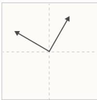
- Directional / linear representation: the hypothesis that features are represented as directions in activation space. If features \(f_1, f_2, \dots\) have scalar activations \(x_{f_1}, x_{f_2},\dots\) and directions \(W_{f_1}, W_{f_2}, \dots\), the layer activation is approximately \[ x_{f_1} W_{f_1} + x_{f_2} W_{f_2} + \dots \] This is not a claim that features are linear functions of inputs — only that the map from features to activations is (approximately) linear.
- Privileged vs non‑privileged bases: a basis is privileged when some architectural choice makes the basis directions special (e.g., an element-wise nonlinearity like ReLU encourages features to align with neurons). Word embeddings and residual streams are often non‑privileged (rotationally symmetric), while MLP layers with ReLU are privileged.
Why does any of this matter? If a basis is privileged and features align with basis directions, neurons can be cleanly interpretable. If the basis is non‑privileged, features may exist as arbitrary directions and we need analysis methods to find them. Superposition pushes features away from basis alignment even when a privileged basis exists, which is part of why polysemantic neurons are so common.
A key intuition from high-dimensional geometry and compressed sensing: although you can only have \(m\) perfectly orthogonal vectors in \(\mathbb{R}^m\), you can have exponentially many almost orthogonal vectors. If features are sparse (rarely active), you can tolerate small cross-talk (interference) between these almost‑orthogonal directions and recover the active features most of the time. That tradeoff is the heart of superposition.
Polysemanticity is what we observe when features don’t align with a neat one-feature‑per‑neuron basis. In high-dimensional space, many almost‑orthogonal directions allow packing many features into fewer neurons.
Demonstrating superposition: the toy autoencoder experiment
The first question the authors tackle is simple and concrete: can a neural network noisily represent more features than it has neurons? To test this they use a highly controlled synthetic experiment.
Setup summary
- Input vector \(x \in \mathbb{R}^n\). Each coordinate \(x_i\) is a “feature.” Each feature has:
- sparsity \(S_i\) (probability of being zero; often they use a common \(S\)),
- importance \(I_i\) (a weight in the training loss).
- If nonzero, \(x_i\) is sampled uniformly from \([0,1]\) (or \([-1,1]\) for some experiments).
- Two model families:
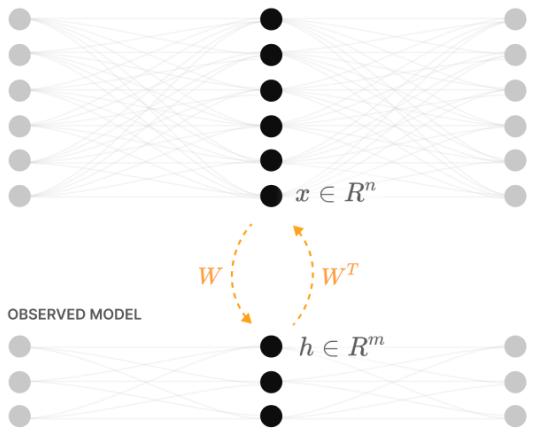
- Linear model: \(h = W x,\; x' = W^\top h + b\). This behaves like a PCA autoencoder.
- ReLU‑output model: \(h = W x,\; x' = \mathrm{ReLU}(W^\top h + b)\). The only difference is the ReLU on the output.
- Loss: weighted MSE, \[ L = \mathbb{E}_x \sum_i I_i (x_i - x'_i)^2. \]
- Key diagnostics:
- Columns \(W_i\) (how each input feature is embedded).
- Gram matrix \(W^\top W\) (shows pairwise overlaps between features).
- Norms \(\|W_i\|\) (whether a feature is represented).
- “Superposition measure”: how much other features project onto \(\hat W_i\).
The punchline
- The linear model always behaves like PCA: it gives each of the top \(m\) principal features their own orthogonal direction and ignores the rest.
- The ReLU‑output model behaves like the linear one when features are dense. BUT as features get sparser, the ReLU model can represent more than \(m\) features by packing them into non‑orthogonal, almost‑orthogonal directions. Initially it uses antipodal pairs (one vector is the negative of another), then more exotic packings as sparsity increases.
Why the ReLU makes a difference
ReLU provides asymmetric treatment of positive and negative interference. If interference would make a dot product negative and therefore be zeroed by ReLU in many sparse cases, that interference becomes “free” (it doesn’t hurt loss). This asymmetry opens a route to pack more features into the same limited dimensions: negative interference is tolerable, positive interference is costly — and with biases the model can turn some small positive interference into effectively negative by shifting thresholds.
The left column shows the linear model’s \(W^\top W\) and feature norms (it picks the top‑m features). The ReLU model on the right starts matching the linear model in the dense regime, then gradually packs more features into superposition as sparsity increases.
This experiment is a clean demonstration that superposition is not just speculation: even in very small ReLU networks trained on simple sparse synthetic data, models will pack more features than they have neurons when doing so is beneficial for loss.
A phase change in representation
One striking finding is that the transition into superposition is not gradual for an individual feature — it behaves like a phase change. For a given feature, training outcomes fall into clear regimes:
- not represented,
- represented with a dedicated (orthogonal) dimension,
- represented in superposition (a fractional share of a dimension).
The authors isolated this with tiny analytic examples. Consider \(n=2\) features, \(m=1\) hidden dimension. There are only a handful of natural candidate solutions:
- \(W=[1,0]\): only feature 1 is represented (feature 2 ignored).
- \(W=[0,1]\): only feature 2 represented.
- \(W=[1,-1]\) (antipodal): both features represented via superposition.
Varying two axes — the sparsity and the relative importance of feature 2 — yields a clear phase diagram. In regions of the parameter space, superposition (the antipodal solution) is the optimal strategy; in others, it is better to ignore the extra feature or give it the dedicated dimension by discarding another feature. The boundaries between these regions are sharp.
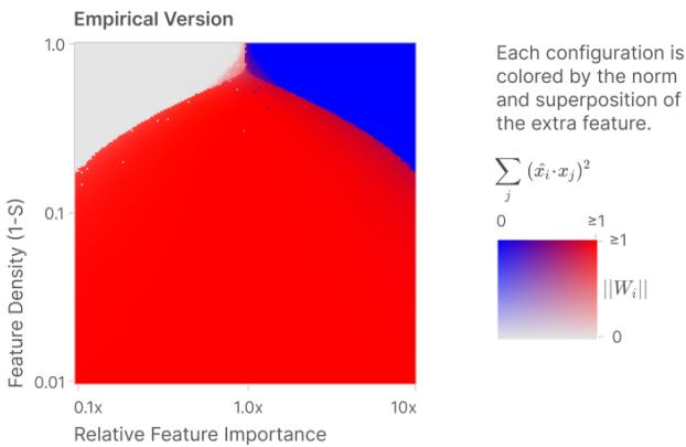
Empirical (left) and theoretical (right) phase diagrams for storing two features in one dimension. The axes are (feature density = \(1-S\)) and relative feature importance. The red area shows where superposition (antipodal solution) is optimal.
The authors extend this analysis to \(n=3, m=2\) and other small combinatorial cases and find matching empirical and theoretical predictions. The upshot: whether a feature ends in superposition or not is governed by a sharp interaction between sparsity and importance.
The geometry of superposition
Once superposition appears, the learned embeddings organize into surprisingly structured geometries — not random scatterings. Under uniform conditions (all features equal importance and sparsity), the optimal arrangements correspond to familiar uniform polytopes: digons (antipodal pairs), triangles, tetrahedra, pentagons, square antiprisms, and so on. The connection to the Thomson problem (placing repelling charges on a sphere) is natural: the model spreads feature vectors to minimize interference, which is analogous to minimizing electrostatic energy.
Key definitions
- Number of features effectively learned: measured by \(\|W\|_F^2 = \sum_i \|W_i\|^2\). If \(\|W_i\|^2 \approx 1\) for represented features and \(\approx 0\) for ignored ones, the Frobenius norm approximates the number of represented features.
- Feature dimensionality: \[ D_i = \frac{\|W_i\|^2}{\sum_j (\hat W_i \cdot W_j)^2}. \] Intuition: what fraction of a hidden dimension does feature \(i\) consume? In an antipodal pair each feature gets \(D=1/2\). These \(D_i\) across features tend to cluster at specific rational fractions corresponding to polytope vertex degrees.
Sticky fractions and polytopes
When plotting \(D_i\) for all features as sparsity changes, the points cluster on horizontal lines — the system prefers a small set of rational fractional dimensionalities. Those fractions match the combinatorial structure of uniform polytopes (e.g., triangles in the plane, tetrahedra in 3D). The learned geometry is not arbitrary: the optimization finds highly symmetric solutions when the data is symmetric.
Deforming the geometry
Breaking uniformity (making one feature denser or more important) deforms the polygon/polytope; sometimes gradually, sometimes causing a sharp snap to a different configuration (a phase change). For example, a regular pentagon can stretch continuously as one feature becomes denser; beyond a threshold it can collapse into two antipodal pairs with the sparse feature ignored — a discontinuous transition corresponding to a swap between two loss minima.
Polytope ↔ low‑rank matrix correspondence
The arrangement of feature vectors (columns of \(W\)) directly determines \(W^\top W\). Rank‑\(m\) positive semi‑definite Gram matrices correspond to point configurations in \(\mathbb{R}^m\) up to rotation. Thus the search over \(W^\top W\) is naturally a search over geometric packings on the unit sphere.
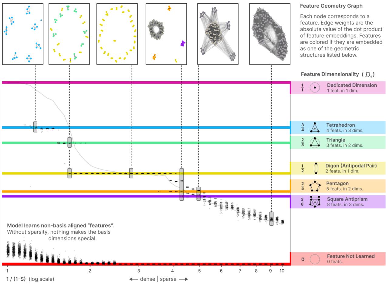
Each dot is a feature’s dimensionality \(D_i\) plotted against sparsity. Horizontal lines correspond to specific geometric packings (digons, triangles, tetrahedra, pentagons,…).
This geometric picture is elegant and somewhat unexpected. It suggests superposition is not just noisy compression — in symmetric situations, it’s a highly structured packing problem with canonical solutions.
Computation while in superposition
So far we’ve seen that networks can store and retrieve features in superposition. But can they compute on those features without decompressing them into a larger representation? The paper answers yes, with a carefully chosen toy: compute \(y = |x|\) elementwise.
Why absolute value?
Absolute value has a small, well-known ReLU decomposition:
\[ |x| = \mathrm{ReLU}(x) + \mathrm{ReLU}(-x). \]This uses ReLU nonlinearity and a small number of neurons per scalar input. If a model can compute absolute value while input features are in superposition, it demonstrates useful computation in superposition and a natural privileged basis (the hidden units must use ReLUs).
Experiment sketch
- Input \(x\) is sparse and can be negative (nonzero entries sampled uniformly from \([-1,1]\)); the target is \(y=|x|\).
- Model: \(h = \mathrm{ReLU}(W_1 x)\), \(y' = \mathrm{ReLU}(W_2 h + b)\). Here \(W_1\) and \(W_2\) are independent (not tied), so the model must learn an internal code.
- Tests: vary \(n\), \(m\), feature sparsity and importance, and inspect the hidden layer weights and neuron semantics.
What happens
- Dense regime: the model learns interpretable circuits — two neurons per input feature (positive and negative sides). Hidden units are largely monosemantic.
- Increasing sparsity: the model begins to pack multiple absolute‑value circuits into the same neurons. Hidden units become polysemantic but still implement reliable computation: they create per‑feature positive/negative detectors in superposition, then recombine.
- Very sparse regime: most or all neurons are highly polysemantic, but the network still approximates absolute value for many features simultaneously.
The important takeaways
- Computation can be performed in superposition, not just storage. The model can route and combine signals from many features even when those features share neurons.
- A privileged basis (hidden ReLU neurons) remains meaningful: features tend to align with neurons more in this setup than in the fully rotation‑invariant case, but alignment is partial and dependent on sparsity.
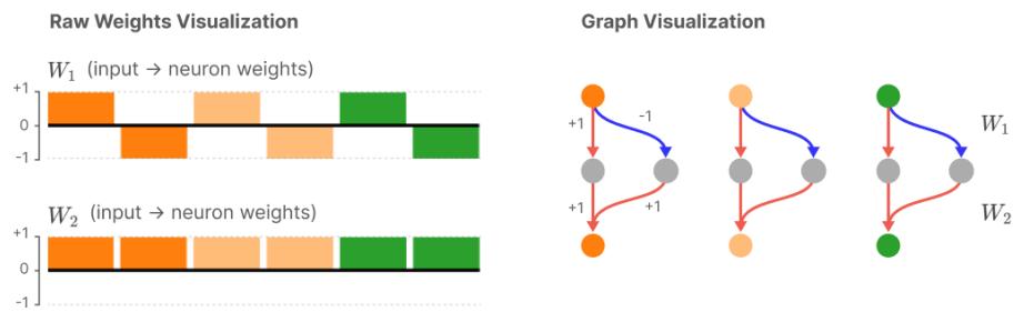
Each panel shows neuron stacks at a different sparsity. The model transitions from mostly monosemantic neurons (top) to heavily polysemantic neurons (bottom), while still computing absolute values.
Mechanistic motif: asymmetric superposition with inhibition
One motif that emerges is asymmetric superposition: one neuron represents features \(a\) and \(b\) with very different magnitudes (e.g., \(W=[2,-1/2]\)), and another neuron uses reciprocal output weights to prioritize one direction while making the other less harmful. To cancel residual positive interference that would be costly, a separate inhibition neuron actively suppresses unwanted activation, effectively turning positive interference into negative (which ReLU can ignore). This pattern is a small but powerful circuit trick for reliable computation in superposition.
Links to adversarial vulnerability
An important consequence of superposition: interference terms (small off‑diagonal entries in \(W^\top W\)) provide natural footholds for adversarial perturbations.
- Non‑superposition, orthogonal case: the effective projection for feature \(i\) looks like \((W^\top W)_i \approx e_i\), a one‑hot vector. Perturbations in other feature directions don’t strongly affect feature \(i\).
- Superposition case: \((W^\top W)_i \approx e_i + \varepsilon\), where \(\varepsilon\) contains many small cross‑terms. An adversary can craft a perturbation combining those cross directions to strongly change the activation of feature \(i\) while keeping a small norm.
Empirically, the authors measure adversarial vulnerability (relative increase in loss under optimal \(L_2\) perturbations) across sparsity regimes and find it tracks the degree of superposition: as the number of features per dimension grows, adversarial vulnerability rises — sometimes by multiple times.
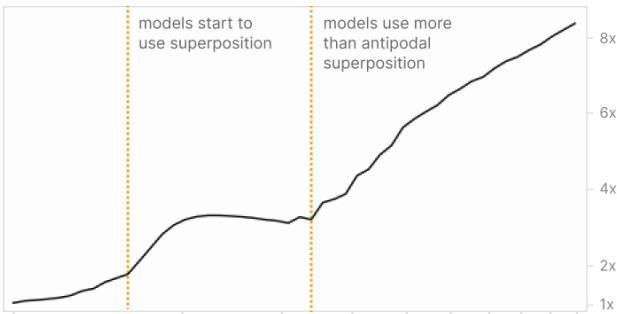
Top: adversarial vulnerability as sparsity increases. Bottom: features per dimension (inverse of average feature dimensionality). Vulnerability closely tracks how crowded each hidden dimension is.
Implications
- Superposition provides an intuitive mechanism for adversarial brittleness: it creates many weak couplings that are exploitable in aggregate.
- This suggests tradeoffs: reducing superposition (via design choices or training regularizers) may improve robustness, but perhaps at a cost in model capacity unless compute or architecture is changed (see strategies below).
What this means for interpretability and safety
Superposition is central to many interpretability headaches:
- If features are basis‑aligned and monosemantic, enumerating features reduces to enumerating neurons — a straightforward path for mechanistic interpretation.
- If features are in superposition, there may be exponentially many features effectively simulated in the network, and they don’t correspond to single neurons. Enumerating them becomes a nontrivial sparse‑coding task.
The authors frame “solving superposition” as any method that enables enumeration or unfolding of a model’s features. Solving it would restore many useful interpretability primitives:
- Decompose activations into pure features across the full distribution.
- Make circuit analysis tractable (weights connecting understandable features).
- Allow more principled safety claims (e.g., sanity checks that specific feature‑circuits are absent).
But solving superposition is hard in large models: it could require massive overcomplete sparse factorizations or architectural changes. Below are three high‑level strategies the paper proposes.
Three strategies to mitigate or solve superposition
- Create models that avoid superposition
- Techniques: heavy L1 sparsity on activations, architectural choices that give more effective neurons per flop (e.g., Mixture‑of‑Experts), or training regimes that punish interference.
- Tradeoffs: likely worse empirical performance unless the architecture provides extra effective capacity (e.g., MoE). Superposition is useful capacity compression for a fixed number of active neurons.
- Post‑hoc decoding: find an overcomplete feature basis
- Treat the hidden activations as compressed measurements and perform sparse coding / compressed sensing to recover feature coordinates.
- Tradeoffs: enormous computational challenge for big models (finding thousands times overcomplete bases), but it leaves the standard model and its performance unchanged.
- Hybrid approaches
- Make small changes during training to reduce superposition or make it easier to decode later (regularizers that bias weight geometry, checkpointing, targeted sparsity).
- Tradeoffs: a middle ground — maybe practical, but needs careful design and empirical validation.
Key practical optimism: superposition seems to be a phase — there exist regimes where it is essentially absent. That means one might be able to design training or architecture strategies to push a model across the phase boundary, at the cost of compute or different engineering tradeoffs.
Limitations and open questions
The toy models are intentionally simple; they are not claims that every phenomenon observed will exactly match large‑scale networks. The work aims to show plausibility, illuminate mechanisms, and offer hypotheses for empirical validation. The paper (and this summary) leave many important open questions:
- How much superposition do real models have? Can we estimate feature sparsity/importance curves in practice?
- Can we design practical algorithms that reliably recover an overcomplete feature basis for real layers?
- How does superposition scale with model size? Does more scale reduce or exacerbate the phenomenon for realistic feature distributions?
- What classes of computation are amenable to efficient implementation in superposition vs. not?
- Can we use compressed sensing theory to derive tight bounds on how many features can be packed for given sparsity and dimensionality?
- Can training regimes (adversarial training, alternative nonlinearities, MoE-style sparsity) shift the phase boundary in a useful way?
The authors also note several empirical replications, independent analyses (e.g., exact solution for \(n=2, m=1\)), and follow‑on results that support the robustness of the main effects.
Closing thoughts
Toy Models of Superposition gives us a new lens for thinking about polysemantic neurons: they are not necessarily bugs or artifacts of training, but sometimes the optimal — or near‑optimal — way to use limited capacity for sparse features. The phenomena are rich:
- Superposition emerges when features are sparse and a nonlinearity allows selective filtering of interference.
- The transition into superposition is often sharp and predictable from sparsity and importance.
- When present, superposition organizes into structured packings (polytopes), not purely random noise.
- Networks can compute while in superposition; neurons need not be monosemantic to participate in robust computation.
- Superposition helps explain some forms of adversarial vulnerability.
For interpretability and safety, this raises both a challenge and a direction. The challenge: superposition complicates naive neuron‑enumeration strategies. The direction: because superposition is a phase phenomenon with structure, there are principled ways (architectural + algorithmic) to either avoid it or decode it.
If you want to explore the experiments yourself, the original paper provides runnable notebooks and code to reproduce key figures. For interpretability researchers, the practical question is not whether superposition exists — now we know it does in plausible regimes — but how much it matters in scale and how to either work with it (decode it) or around it (architectures that reduce it). Both paths look scientifically interesting and practically important.
Further reading
- The original paper: Elhage et al., “Toy Models of Superposition” (2022).
- Related topics: compressed sensing, disentanglement literature, mechanisms of adversarial examples.
Acknowledgement
This article is a condensed, pedagogical walk‑through of Elhage et al.’s paper intended to clarify the main ideas, experiments, and implications. For details, proofs, extended results, and code, consult the original paper and its supplemental notebooks.