](https://deep-paper.org/en/paper/2305.00316/images/cover.png)
Imagine teaching a child to recognize cats. They learn perfectly. Then you teach them to recognize dogs — and suddenly, they can’t identify a cat anymore. This puzzling scenario is a daily reality for artificial intelligence. It’s called catastrophic forgetting: when a machine learning model learns a new task, it often overwrites what it previously knew, causing a dramatic drop in performance.
This is the central challenge of continual learning (also known as lifelong learning): how can we build intelligent systems that learn new skills sequentially without forgetting old ones? Over the years, researchers have developed many practical strategies to combat this problem, generally falling into three main camps:
- Memory-based methods: store samples from old tasks and mix them with new data (often called rehearsal).
- Regularization-based methods: add penalty terms to the objective to keep parameters aligned with previously learned tasks.
- Expansion-based methods: grow the network architecture to accommodate new knowledge.
While these methods have made continual learning better in practice, the field has lacked a unifying theory. Are these strategies fundamentally different, or are they variations of a common principle? And how exactly does memory replay (rehearsal) affect a model’s ability to generalize rather than overfit?
A recent research paper — “The Ideal Continual Learner: An Agent That Never Forgets” — takes on these questions with a bold goal: to define a mathematically perfect learner that never forgets, by design. Using this theoretical construct, the authors reveal deep connections between continual learning, multitask learning, optimization theory, and even classical control systems.
Let’s unpack what it takes to design an ideal learner with perfect memory.
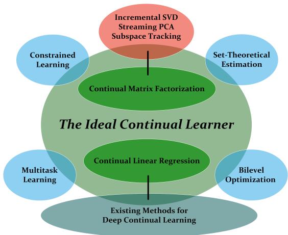
Figure 1: The Ideal Continual Learner (ICL) acts as a hub connecting diverse fields such as multitask learning, bilevel optimization, and constrained learning.
The Ground Rules for Never Forgetting
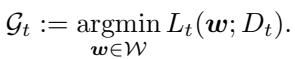
In continual learning, tasks arrive sequentially — \(t = 1, 2, \ldots, T\). Each task has its own dataset and objective function \(L_t(\boldsymbol{w})\) to minimize, where \( \boldsymbol{w} \) represents the model’s parameters. The set of all global minimizers for task \(t\) is denoted \( \mathcal{G}_t \).
The holy grail is to find a single \( \boldsymbol{w} \) that performs optimally for all tasks. To make this possible, the paper introduces a foundational assumption:
Assumption 1 (Shared Multitask Model): There exists at least one common global minimizer across all tasks — mathematically,
\[ \bigcap_{t=1}^{T} \mathcal{G}_t \neq \emptyset. \]This assumption may be strong, but it’s essential. If the intersection of all solution sets were empty, then forgetting would be unavoidable — no model could satisfy every task at once. By assuming that a shared solution exists, the authors can focus on how to efficiently discover and preserve it.
This also bypasses a key computational barrier: determining whether the intersection of global minimizers exists is an NP-hard problem. The shared multitask model assumption makes the ideal continual learner tractable for theoretical analysis.
Defining the Ideal Continual Learner (ICL)
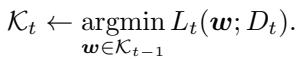
With the stage set, the definition of ICL is remarkably simple but profound. It works recursively: starting from the entire space of possible models (\(\mathcal{K}_0 = \mathcal{W}\)), ICL learns task 1 and stores all its optimal solutions (\(\mathcal{K}_1 = \mathcal{G}_1\)). When learning task 2, it only searches within these previously optimal solutions — then for task 3, it searches within the intersection of all prior sets, and so on.
Formally,
\[ \mathcal{K}_t = \operatorname*{argmin}_{\boldsymbol{w} \in \mathcal{K}_{t-1}} L_t(\boldsymbol{w}). \]This creates a nested sequence:
\[ \mathcal{W} = \mathcal{K}_0 \supseteq \mathcal{K}_1 \supseteq \mathcal{K}_2 \supseteq \cdots \supseteq \mathcal{K}_T. \]You can think of \( \mathcal{K}_t \) as the learner’s knowledge state — a progressively refined representation containing everything it has learned so far. Like a human expert who compresses volumes of study material into a few essential formulas, ICL keeps only what is necessary yet never loses what came before.
The “ideal” in Ideal Continual Learner reflects its theoretical nature. Computing all global minimizers is infeasible for complex neural networks, but treating it as an abstract construct lets researchers derive powerful insights about how practical learners should behave.
The Properties of a Perfect Learner
ICL exhibits two key attributes that make forgetting impossible:
Sufficiency — It Never Forgets. Under the shared multitask assumption, ICL’s solution set at step \(t\) equals the intersection of all prior tasks’ solutions:
\[ \mathcal{K}_t = \bigcap_{i=1}^t \mathcal{G}_i. \]Every point within \( \mathcal{K}_t \) remains optimal for all previous tasks, guaranteeing perfect retention.
Minimality — It Stores Exactly What’s Needed. The learner must preserve complete information about its solution space. If it stores only a subset or partial representation, future compatible solutions could be lost. Retaining the full set (or equivalent information like gradient equations) is the minimal condition for zero forgetting.
This makes ICL not only optimal but information-theoretically efficient: storing less leads to forgetting; storing more is unnecessary.
Unifying the Landscape: ICL in Disguise
The beauty of ICL lies in its versatility. The paper proves that this single recursive definition elegantly mirrors several familiar frameworks in machine learning.
ICL as a Bilevel Optimizer
Each step of ICL solves an upper-level optimization constrained by lower-level conditions derived from prior tasks — a form of bilevel optimization.
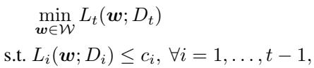
At every step:
\[ \min_{\boldsymbol{w}} L_t(\boldsymbol{w}) \quad \text{s.t.} \ L_i(\boldsymbol{w}) \le c_i, \ \forall i < t, \]where \( c_i \) is the minimal loss from task \(i\).
For convex objectives, these constraints are equivalent to requiring zero gradients from all prior tasks — ensuring that the learner doesn’t “unlearn” them.
Storing gradients or minimal losses provides enough information to resist forgetting.
ICL as a Multitask Learner
Perhaps the most surprising connection is to multitask learning, where all tasks are trained simultaneously via a combined loss:
\[ \sum_{i=1}^{t} \alpha_i L_i(\boldsymbol{w}), \]with positive weights \( \alpha_i \).
When a shared solution exists, the sequential ICL procedure recovers the same optimal set as multitask learning.
This resolves a long-standing debate: under the right assumptions, continual learning and multitask learning yield equivalent outcomes. Sequential learning doesn’t have to be a compromise; it can be just as powerful.
ICL in Practice: Two Key Examples
The paper grounds the theory in two illustrative cases that connect directly to how deep continual learning is done practically.
Example 1: Continual Linear Regression
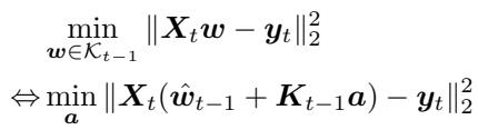
Each task aims to fit a linear model minimizing \(L_t(\boldsymbol{w}) = \|X_t \boldsymbol{w} - y_t\|_2^2\). The solution set \(\mathcal{G}_t\) forms an affine subspace.
A traditional method alternates projections between these subspaces (Figure 2a) — simple but often forgetful. ICL instead solves the first task, stores its full solution subspace, and constrains subsequent optimization to remain compatible with it (Figure 2b).
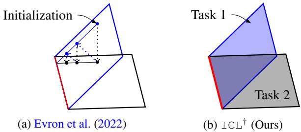
Figure 2: Unlike alternating projection approaches, ICL systematically restricts new optimizations to the intersection of known solution spaces.
To implement this, ICL stores a particular solution \( \hat{\boldsymbol{w}}_{t-1} \) and an orthonormal basis \( \boldsymbol{K}_{t-1} \) spanning the shared nullspace of previous data matrices. Any valid solution takes the form \( \boldsymbol{w} = \hat{\boldsymbol{w}}_{t-1} + \boldsymbol{K}_{t-1} \boldsymbol{a} \), turning each new task into a smaller optimization over the coefficients \( \boldsymbol{a} \).
Reducing the search space to new coefficients enables compact storage and efficient updates.
This mechanism mirrors orthogonal gradient descent (OGD) — a popular deep learning method that projects gradients into safe directions. The paper shows that OGD is essentially performing gradient descent on ICL’s objective, linking this practical technique to its theoretical foundation.
Example 2: Continual Matrix Factorization
Another example involves matrix decomposition, \( Y_t \approx UC \), akin to Principal Component Analysis (PCA). Each task adds new data represented by a subspace \(S_t\).
ICL seeks an orthonormal basis capturing the sum of all learned subspaces:
\[ \sum_{i=1}^t S_i. \]When a new task arrives:
- The data \(Y_t\) is projected onto the orthogonal complement of the old subspace to reveal new information.
- An SVD computes an orthonormal basis for that new space.
- The overall basis expands by concatenating this update.
This expansion-based view provides a principled explanation for why wider neural networks forget less — each column added corresponds to new, independent knowledge. Instead of fixed-width networks, ICL gives exact mathematical guidance for when and how to expand.
From a Perfect Optimizer to a Real Learner
ICL doesn’t just work as an optimizer; the paper extends it into the domain of statistical learning theory, where data is drawn from distributions. It distinguishes between empirical solution sets (based on training samples) and true solution sets (based on underlying distributions).
Under standard Lipschitz and boundedness assumptions, the authors derive generalization bounds that quantify how well ICL approximates the ideal learner in expectation.
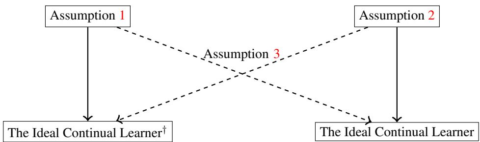
Figure 3: Theoretical connections between empirical and true learners. Dashed arrows represent approximate guarantees under standard generalization assumptions.
Two key results emerge:
- Theorem 1: The empirical version of ICL (\( \text{ICL}^\dagger \)) is approximately optimal for all true tasks when Assumption 1 holds.
- Theorem 2: A relaxed version of ICL allows small deviations in earlier tasks and remains approximately optimal, ensuring feasibility in practice.
The Theory Behind Rehearsal
One of the most debated topics in continual learning is whether rehearsal — replaying stored examples from previous tasks — truly helps generalization or merely prevents forgetting through brute force.
ICL settles this debate with a rigorous bound.
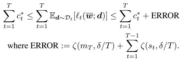
The generalization error is provably reduced when more samples are stored for rehearsal.
Formally, the total generalization error decreases proportionally to the number of samples \(s_t\) retained for each prior task:
\[ \text{ERROR} = \zeta(m_T, \delta/T) + \sum_{t=1}^{T-1} \zeta(s_t, \delta/T), \]where \(\zeta(\cdot)\) quantifies statistical uncertainty. More stored samples → smaller error.
Importantly, the bound depends only on how many samples are kept, not which ones. This matches empirical results showing that random sampling is often as effective as complex memory-selection strategies. In other words, quantity trumps cleverness when the samples are i.i.d.
Conclusion: All Roads Lead to ICL
The Ideal Continual Learner provides a unifying theoretical foundation for lifelong learning. Its insights include:
- A Common Principle: Memory-based, regularization-based, and expansion-based methods are all practical approximations of ICL.
- Deep Connections: The framework connects continual learning with multitask learning, bilevel optimization, constrained learning, and control theory.
- Quantitative Understanding: It offers the first rigorous generalization bounds for rehearsal and explains why expanding network capacity prevents forgetting.
While ICL in its exact form is not computationally realizable, its theoretical blueprint guides how future algorithms can mimic a learner that never forgets. It shows that continual learning isn’t an endless struggle against forgetting; it’s a journey toward approximating this ideal — an agent with perfect memory and infinite adaptability.