](https://deep-paper.org/en/paper/2306.11908/images/cover.png)
Introduction
In the world of modern machine learning, we have moved past the era of simply predicting an “average.” Whether in personalized medicine, computational advertising, or public policy, the most valuable insights often lie in heterogeneity—understanding how an effect varies across different subgroups of a population.
For example, a new drug might have a modest average effect on a population but could be life-saving for one genetic subgroup and harmful to another. A straightforward regression model typically misses these nuances.
To solve this, researchers turn to Generalized Random Forests (GRF). This framework, popularized by Athey et al., is the gold standard for estimating heterogeneous treatment effects and varying coefficients. It adapts the powerful random forest algorithm to solve statistical estimating equations locally.
However, GRF has a bottleneck. The standard algorithm relies on a gradient-based splitting criterion that requires inverting a matrix (the Jacobian) at every step of tree growth. In high-dimensional settings, or when features are highly correlated, this process becomes computationally expensive and numerically unstable.
In this post, we explore a new method proposed by Fleischer, Stephens, and Yang: Fixed-Point Trees (FPT). This approach replaces the expensive gradient step with a fixed-point approximation. The result? A method that is significantly faster, more stable, and just as accurate as the original—unlocking scalable causal inference for larger, more complex datasets.
The Context: Generalized Random Forests
To understand the innovation of Fixed-Point Trees, we first need to understand what Generalized Random Forests (GRF) are trying to achieve.
Standard Random Forests are designed to minimize prediction error (like Mean Squared Error for regression). GRFs are more ambitious. They aim to estimate a parameter of interest, \(\theta^*(x)\), which is defined as the solution to a local estimating equation:
Here, \(\psi\) is a “score function.” For example, in a quantile regression, \(\psi\) would be a check function; in instrumental variables, it involves covariance moments. The goal is to find the \(\theta\) that makes the expected score zero, conditional on the features \(X\).
GRF works in two stages:
- Stage I (Tree Training): The algorithm builds a forest of trees to partition the data into “leaves” where the observations are similar.
- Stage II (Estimation): For a new test point \(x\), the forest calculates weights \(\alpha_i(x)\) based on how often training example \(i\) falls into the same leaf as \(x\).
The final estimate is found by solving the weighted equation shown above. The magic of GRF lies in Stage I: how do we build a tree that groups “similar” data points when the target \(\theta\) isn’t directly observable (like a treatment effect)?
The Bottleneck: Gradient-Based Splitting
The core of any decision tree is the splitting rule. The tree looks at a parent node \(P\) and tries to split it into two children, \(C_1\) and \(C_2\), to maximize the difference (heterogeneity) between the parameters in the two children.
Ideally, we would maximize a criterion \(\Delta(C_1, C_2)\) based on the true parameter values in the children nodes:
Since we don’t know the true parameters \(\hat{\theta}_{C_1}\) and \(\hat{\theta}_{C_2}\) ahead of time (calculating them for every possible split is too slow), standard GRF uses a Gradient-Based Approximation. It approximates the parameters in the children by taking a single Newton-Raphson step from the parent’s parameter \(\hat{\theta}_P\).
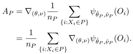
This approximation leads to the “Grad” estimator:
The Problem with the Gradient
Look closely at the equation above. The term \(A_P^{-1}\) represents the inverse of the Jacobian matrix. The Jacobian \(A_P\) measures the curvature of the score function:
Relying on \(A_P^{-1}\) introduces two major problems:
- Computational Cost: Inverting a matrix scales cubically, \(O(K^3)\), where \(K\) is the dimension of the parameter \(\theta\). If you are estimating a complex model with many parameters, this step becomes agonizingly slow.
- Instability: If your features are highly correlated (multicollinearity), the matrix \(A_P\) becomes “ill-conditioned” (nearly singular). Inverting it leads to massive numerical explosions, causing the split criterion to behave erratically.
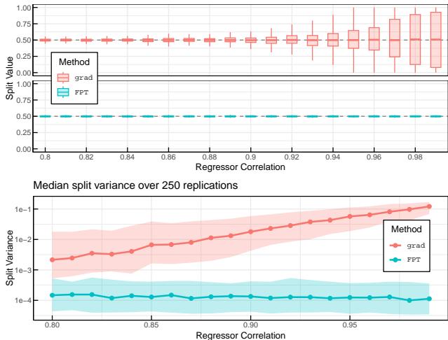
The authors demonstrate this instability in Figure 1. The plots below show what happens when regressors are highly correlated. The “grad” method (orange) produces high-variance splits, fluctuating wildly. The proposed “FPT” method (blue) remains perfectly stable.
The Solution: Fixed-Point Trees
The researchers propose a method that eliminates the need for the inverse Jacobian entirely. They call it the Fixed-Point Tree (FPT) algorithm.
The Intuition
Instead of viewing the parameter estimation as a root-finding problem requiring a Newton step (which needs a derivative/Jacobian), they reframe it as a fixed-point iteration.
Standard fixed-point theory suggests that under certain conditions, we can approximate a solution by iteratively applying a function. The authors propose approximating the child parameters \(\theta_{C_j}\) by taking a “step” from the parent parameter \(\theta_P\) in the direction of the negative score, scaled by a constant \(\eta\), without rotating it by the inverse Jacobian.
The FPT approximation looks like this:
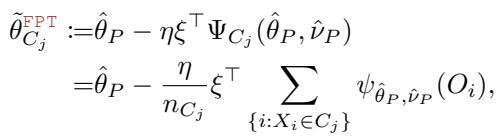
Compare this to the gradient formula in the previous section. The expensive matrix \(A_P^{-1}\) is gone, replaced by a scalar \(\eta\) and a selector matrix \(\xi\). This seemingly simple change reduces the computational complexity from \(O(K^3)\) to essentially \(O(K)\).
Does it find the same splits?
You might worry that removing the Jacobian changes the “direction” of the gradient, leading to suboptimal splits. However, for the purpose of a decision tree, we only care about the ranking of the splits. We need to know which split is better, not the exact magnitude of the improvement.
The authors prove that the FPT criterion is asymptotically equivalent to an “oracle” criterion weighted by the Jacobian. More intuitively, Figure 2 shows the value of the splitting criterion across different split thresholds.
![Figure 2: Criterion values across candidate splits (C_1(t), C_2(t)) over threshold t in [0, 1]. The location of the optimal split under each criterion is given by the corresponding vertical line.](/en/paper/2306.11908/images/030.jpg#center)
Notice that while the curves have different heights (scales), their peaks—the optimal split points—align almost perfectly. This means FPT finds effectively the same structure as the computationally expensive gradient method.
Implementation: The Pseudo-Outcome Trick
To implement this efficiently, GRF uses “pseudo-outcomes.” The idea is to transform the complex parameter estimation problem into a standard regression problem. We calculate a “fake label” (pseudo-outcome) for every data point and then run a standard CART (Classification and Regression Tree) algorithm on those labels.
For the standard Gradient method, the pseudo-outcome \(\rho_i^{\text{grad}}\) involves the inverse Jacobian:
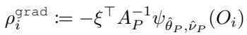
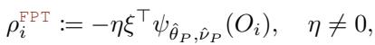
For the Fixed-Point method, the pseudo-outcome \(\rho_i^{\text{FPT}}\) simplifies to the negative score function:
The algorithm simply calculates these residuals at the parent node and feeds them into a standard regression tree splitter. This allows the use of highly optimized tree-building libraries.
Application: Heterogeneous Treatment Effects
One of the most popular uses of GRF is estimating Heterogeneous Treatment Effects (HTE). In this setting, we have an outcome \(Y\), a treatment \(W\), and covariates \(X\). We want to know how the effect of \(W\) on \(Y\) changes based on \(X\).
The model is often structured as:

Here, \(\theta^*(x)\) represents the treatment effect.
Using the FPT approach, we can define specific pseudo-outcomes for this model that are extremely fast to compute. The authors introduce a specific acceleration for these linear models using a “one-step” approximation for the parent parameters as well, further reducing overhead.
The pseudo-outcome for the FPT approach in this setting essentially becomes the interaction between the regressor and the residual:
This avoids the \(O(K^3)\) cost entirely, which is a game-changer when testing multiple concurrent treatments (e.g., A/B/n testing with many arms).
Experimental Results
The theoretical benefits are clear, but how does FPT perform in practice? The authors conducted extensive simulations on both Varying Coefficient Models (VCM) and Heterogeneous Treatment Effects (HTE).
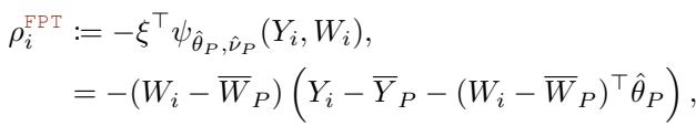
1. Computational Speed
The primary claim of the paper is speed. Figure 3 shows the speedup factor of FPT compared to the standard Gradient method as the dimension of the target parameter (\(K\)) increases.
As the dimension \(K\) grows (from 4 to 256), the speedup becomes massive—FPT is over 3.5x faster in high-dimensional settings. Even for lower dimensions, there is a consistent performance gain.
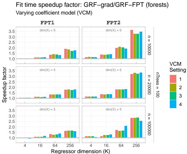
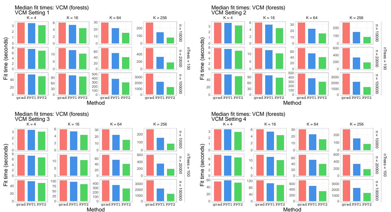
Looking at the absolute fit times in Figure 5, we see that while the gradient method (red) explodes in time as \(K\) increases, the FPT methods (green and blue) remain efficient.
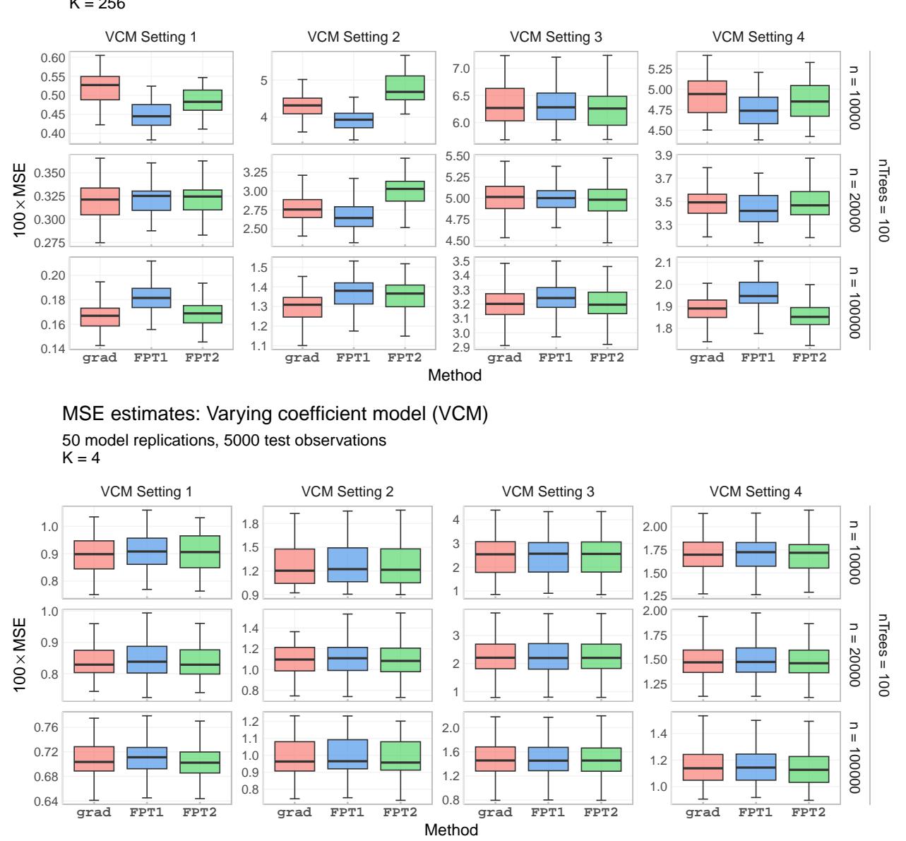
2. Statistical Accuracy
Speed is useless if the estimates are wrong. The authors measured the Mean Squared Error (MSE) of the parameter estimates.
Figure 6 compares the MSE of the Gradient method against FPT. The curves largely overlap, indicating that FPT sacrifices virtually no statistical accuracy for its speed gains. In some high-dimensional cases (top row), FPT actually performs slightly better, likely due to the numerical stability issues of the gradient method discussed earlier.
3. Real-World Data: California Housing
To illustrate the method on real data, the authors applied FPT to the famous California Housing dataset. They modeled housing prices as a function of various features (income, bedrooms, population), allowing the coefficients of these features to vary geographically (by latitude and longitude).
This is a classic “Varying Coefficient Model.” The resulting maps (Figure 4) show distinct geographic patterns.
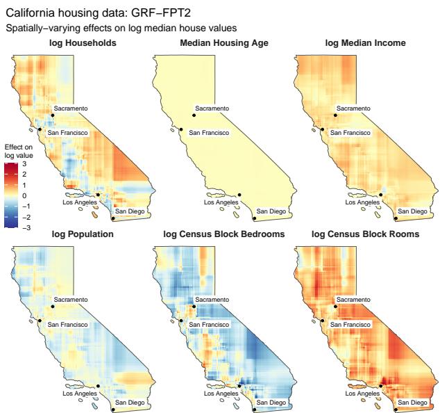
For example, look at the effect of “log Households” (top left). In dense urban centers (Los Angeles, SF), the effect is negative (red/orange)—more crowding might lower value. In rural areas (blue), the effect is positive—more neighbors might signal a desirable community. The FPT algorithm captured these complex spatial heterogeneities efficiently.
Conclusion
Generalized Random Forests have transformed how we analyze heterogeneous effects, but their reliance on Jacobian inversion has been a lingering drag on performance and stability.
The Fixed-Point Tree (FPT) algorithm removes this barrier. By swapping the gradient-based splitting criterion for a fixed-point approximation, FPT offers:
- Speed: Eliminates \(O(K^3)\) matrix inversions, achieving multi-fold speedups.
- Stability: Removes sensitivity to multicollinearity and ill-conditioned matrices.
- Accuracy: Maintains the rigorous consistency and asymptotic normality guarantees of the original GRF.
For practitioners and researchers working with high-dimensional data or complex causal models, FPT turns a computationally heavy task into a scalable workflow. It allows us to ask more complex questions—estimating effects across many treatments or features—without waiting days for the answers.