Beyond Neurons: Finding the True Features in Language Models with Sparse Autoencoders

Large Language Models (LLMs) like GPT-4 have demonstrated astonishing capabilities, but a fundamental question remains—how do they actually work? We can see their inputs and outputs, but the internal reasoning behind their predictions is buried inside billions of parameters. This opacity is a major obstacle to building systems that are safe, fair, and trustworthy. If we don’t understand why a model makes a decision, how can we correct or prevent harmful behavior?

A key difficulty in opening this “black box” is a phenomenon called polysemanticity. This happens when a single neuron activates in response to multiple, unrelated concepts. For example, the same neuron might respond to the word “king,” an image of a lion, and a snippet of Python code—all at once. Trying to interpret models neuron by neuron is like trying to understand a novel by looking at individual letters that form thousands of different words—it’s bewildering.

Researchers believe polysemanticity stems from superposition—the idea that neural networks represent more distinct features than they have neurons to store them. To cope, models encode multiple features into directions within a high‑dimensional activation space, rather than one per neuron. A single concept may be represented as a specific pattern of activations distributed across many neurons.

This is where the recent paper Sparse Autoencoders Find Highly Interpretable Features in Language Models breaks new ground. The authors propose an unsupervised method to disentangle these superimposed features. Using sparse autoencoders, they learn a “dictionary” of underlying features, moving beyond neurons to uncover the true building blocks of a model’s understanding. The outcome: features that are vastly more interpretable and tightly linked to a model’s behavior—offering a promising path toward genuine transparency.

From a Tangled Web of Neurons to a Dictionary of Features

To make sense of complex systems, we must decompose them into their fundamental parts. In LLMs, those parts are usually neurons—but neurons are plagued by polysemanticity. The goal of this work is to find a better set of components: a dictionary of monosemantic features, where each feature corresponds to a single, human‑understandable concept.

The foundation of their method is sparse dictionary learning, a well‑known idea in signal processing and neuroscience. It assumes any complex signal—in this case, the internal activations of a language model—can be reconstructed from only a few elements of a larger dictionary.

Imagine describing the color “burnt sienna.” You could specify its RGB values (precise but meaningless to most humans) or say “mostly red, with touches of yellow and black.” Sparse dictionary learning takes the second approach: combining a few simple elements to represent something intricate.

The team applied this principle directly to language model activations. Using a sparse autoencoder, they learned a dictionary of high‑level features, as illustrated below.

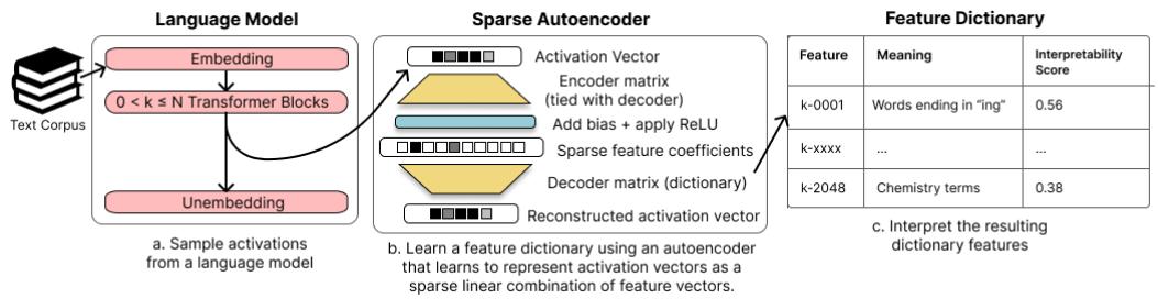
Figure 1: The authors sample activations from a language model, train a sparse autoencoder to learn a feature dictionary, and interpret the resulting features using automated methods.

The Core Mechanism: Learning Features with Sparse Autoencoders

An autoencoder is a neural network with two parts—an encoder that compresses input data and a decoder that reconstructs it. The insight here lies in how sparsity is enforced during training.

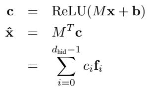
Figure 2: The sparse autoencoder encodes activations into sparse feature coefficients and reconstructs them as a weighted sum of learned dictionary features.

Here’s the intuition:

• Input vector \( \mathbf{x} \): A sample of activations from a transformer layer.
• Encoder matrix \( M \): Each row acts as a detector for a specific feature.
• Bias \( \mathbf{b} \): Adds offset before activation.
• Coefficients \( \mathbf{c} = \operatorname{ReLU}(M\mathbf{x} + \mathbf{b}) \): Sparse vector of feature activations—most values are zero.
• Decoder \( M^T \): Transposed encoder. Each column \( \mathbf{f}_i \) is a learned dictionary feature.
• Reconstruction \( \hat{\mathbf{x}} = M^T\mathbf{c} \): A sparse linear combination of dictionary features approximating the original activations.

Training minimizes two competing objectives:

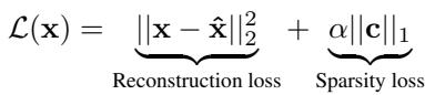
Figure 3: The autoencoder loss combines a reconstruction term ensuring fidelity and a sparsity term promoting simplicity.

1. Reconstruction Loss \( \|{\mathbf{x}} - \hat{{\mathbf{x}}}\|_{2}^{2} \): Encourages the network to accurately rebuild the input.
2. Sparsity Loss \( \alpha \|{\mathbf{c}}\|_{1} \): Penalizes the number of active features. The hyperparameter \( \alpha \) balances fidelity with simplicity.

This dynamic forces the decoder features to become meaningful, disentangled directions—the minimal set of building blocks that explain the data.

Are These Features Useful and Interpretable?

To assess interpretability, the authors needed a scalable, objective metric. They adopted OpenAI’s auto‑interpretation protocol (Bills et al., 2023), which leverages LLMs themselves to rate how understandable a feature’s behavior is.

The process:

1. Identify text snippets where a feature activates strongly.
2. Ask GPT‑4 to describe what that feature is detecting.
3. Ask GPT‑3.5 to simulate the feature’s activations on new text using that description.
4. Measure the correlation between predicted and actual activations—the interpretability score.

An example of feature descriptions and scores is shown below.

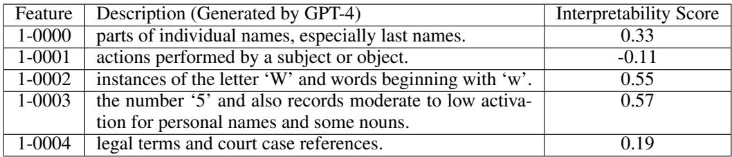
Table 1: Sample dictionary features from the residual stream of Pythia‑70M with GPT‑4‑generated descriptions and automated interpretability scores.

When compared to other decomposition techniques such as PCA, ICA, or the raw neuron basis, sparse autoencoders vastly outperform them.

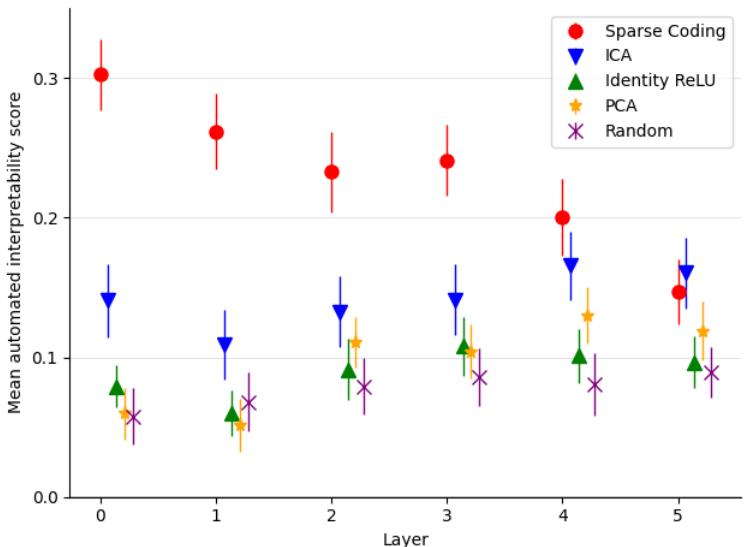
Figure 4: Mean automated interpretability scores across layers. Sparse coding achieves the highest interpretability at nearly every layer.

The result: sparse features are significantly more interpretable than those found by standard methods, suggesting that they reveal genuine semantic structure within the model.

Pinpointing Causal Behavior in Model Computations

Interpretability is one thing—causality is another. Do these features actually cause certain behaviors in the model?

To test this, the authors used a canonical challenge: Indirect Object Identification (IOI). Given a sentence such as “Then, Alice and Bob went to the store. Alice gave a snack to ____,” the model should predict “Bob.”

Using activation patching, a causal intervention method, they examined how altering internal activations along these learned feature directions affects output predictions.

1. Base run: Model predicts “Bob.”
2. Target run: Replace “Bob” with “Vanessa.”
3. Patching run: Re‑execute on the base input, but at a chosen layer, replace the activations of selected features with those from the target run.

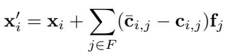
Equation: The patched activation \( \mathbf{x}' = \mathbf{x} + \sum_{j \in F} (\hat{\mathbf{c}}_j - \mathbf{c}_j)\mathbf{f}_j \) modifies internal representations along chosen feature directions.

The effectiveness of patching is measured by the KL divergence between the model’s output distributions on the patched versus target sentences.

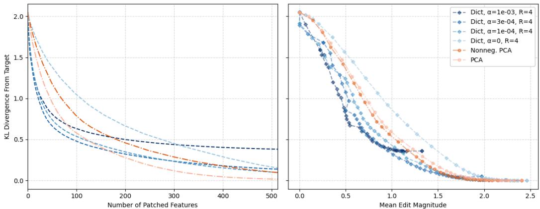
Figure 5: Sparse dictionaries achieve equivalent causal edits with fewer patched features and smaller total edit magnitudes than PCA.

Sparse features enable far more precise interventions—achieving the same behavioral change with fewer features and smaller magnitudes. They cleanly isolate the features that drive specific tasks, proving that these directions are causally meaningful representations within the model.

Peering Inside: Case Studies of Individual Features

Beyond aggregate metrics, the paper showcases examples of individual dictionary features to highlight their monosemanticity—each represents a single, comprehensible concept.

An “Apostrophe” Feature

One striking example is a feature that activates almost exclusively on apostrophes.

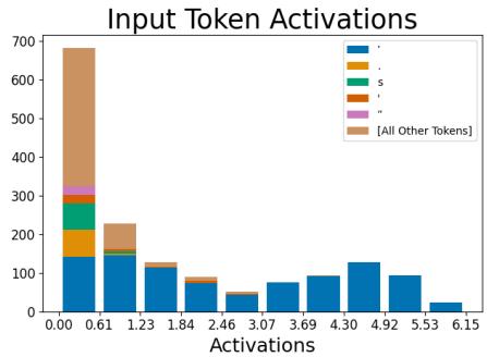
Figure 6: Left—activations cluster almost entirely on apostrophe tokens. Right—ablating this feature primarily suppresses predictions of the following “s” token.

When the researchers removed (ablated) this feature, the model became less likely to generate “’s”—precisely what one expects given its linguistic role in possessives and contractions. This demonstrates a clean, human‑interpretable causal mapping between internal representation and output behavior.

Automatically Discovering Circuits

Perhaps the paper’s most exciting contribution is how sparse features can reveal circuits—chains of features that interact across layers.

The team targeted a feature predicting closing parentheses “)”. By systematically ablating previous‑layer features and measuring the effect on this target’s activation, they built a causal graph of dependencies.

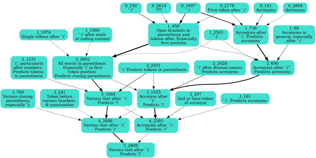
Figure 7: An automatically discovered circuit for the “closing parenthesis” feature. Early layers detect opening brackets or acronyms; later layers integrate these signals to predict the closing parenthesis.

This circuit beautifully mirrors human reasoning: layer 0 recognizes “(”, middle layers interpret text within parentheses, and the final layer predicts “)”. Sparse autoencoders thus provide the scaffolding for tracing model computations feature‑by‑feature.

Why This Matters: Toward Transparent Language Models

This research is a major step toward mechanistic interpretability—understanding models in terms of individual computational units with clear semantics.

Key Takeaways

• Superposition can be resolved. Sparse autoencoders disentangle overlapping features into distinct, sparse directions.
• Features are more interpretable than neurons. Automated tests consistently show higher interpretability scores.
• Features are causally relevant. They can precisely mediate tasks like the IOI challenge, enabling fine‑grained control.

While reconstruction of activations isn’t perfect, and the method currently works best for the residual stream rather than deeper MLP layers, these limitations define clear avenues for future research. Improving reconstruction fidelity or extending sparse feature discovery to other components could give us an even clearer map of what our models compute internally.

Mechanistic interpretability’s long‑term goal—sometimes called enumerative safety—is to produce a human‑understandable catalog of every feature a model uses, providing assurance it cannot perform harmful or deceptive behaviors. Sparse autoencoders offer a scalable, unsupervised path toward that vision.

By replacing neurons with interpretable features, this work gives us a sharper lens on model internals—paving the way toward AI systems whose computations we can finally see, understand, and guide.