](https://deep-paper.org/en/paper/2310.08731/images/cover.png)
Imagine you have trained a robot to navigate a maze. It has spent millions of simulation steps learning that “red tile means lava” and “green tile means goal.” It is perfect. Then, you deploy it into the real world. Suddenly, the lighting changes, or a door that was always open is now locked, or the floor becomes slippery.
In Reinforcement Learning (RL), this is known as novelty—a sudden, permanent shift in the environment’s dynamics or visuals that the agent never anticipated during training.
Typically, when an RL agent encounters something it hasn’t seen before, it fails catastrophically. It might run in circles, crash, or confidently take dangerous actions because its internal policy is no longer valid. To prevent this, we need Novelty Detection: a system that acts as a “check engine” light, warning the agent that the world has changed and it should probably stop or adapt.
Today, we are diving deep into a research paper titled “Novelty Detection in Reinforcement Learning with World Models.” This work proposes a fascinating, mathematically grounded way to detect these changes without relying on the messy, manual “thresholds” that plague traditional methods.
The Problem with “Surprise”
Before we get to the solution, we have to understand why this is hard. In standard machine learning, anomaly detection is often treated as a “distribution shift.” You look at the data coming in, and if it looks statistically different from your training data, you flag it.
In RL, however, the data is not static. The agent is moving, the “camera” is panning, and the states are constantly changing based on actions. A standard approach is to measure prediction error. If the agent predicts the next state and gets it wrong, is that a novelty?
Not necessarily. It might just be stochastic noise (aleatoric uncertainty). Or perhaps the agent is in a corner of the map it rarely visited (epistemic uncertainty).
Most existing methods, such as RIQN (Recurrent Implicit Quantile Networks), solve this by setting a manual threshold. You pick a number, say \(0.5\). If the error score is above \(0.5\), it’s a novelty. But how do you choose that number? It requires you to know what a novelty looks like before it happens, which contradicts the very definition of an “unanticipated” novelty.
The authors of this paper ask a better question: Can we use the agent’s own understanding of the world to define a dynamic boundary for novelty, without human tuning?
The Core Concept: World Models
To understand the method, we first need to understand the architecture it is built upon: the World Model. Specifically, this paper uses DreamerV2.
In traditional RL, an agent looks at an image (\(x_t\)) and outputs an action (\(a_t\)). A World Model goes a step further. It tries to learn a compact, internal representation of the world. It consists of:
- Encoder: Turns the high-dimensional image \(x_t\) into a compact latent state \(z_t\).
- Recurrent Model: Maintains a “history” \(h_t\) based on past states and actions.
- Predictor: Guesses what happens next.
Crucially, DreamerV2 uses a Variational Autoencoder (VAE) setup. It balances two distributions:
- The Posterior: \(p(z_t | h_t, x_t)\). This is the agent’s understanding of the state after seeing the actual image \(x_t\).
- The Prior: \(p(z_t | h_t)\). This is the agent’s prediction of the state based only on its history \(h_t\), before seeing the image.
During training, the agent minimizes the difference (KL Divergence) between the Prior and the Posterior. It tries to make its predictions (Prior) as good as its observations (Posterior).
The loss function for training looks like this:
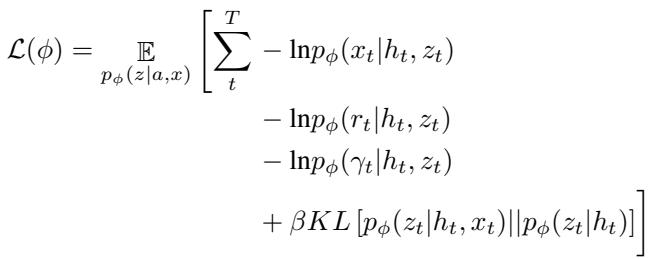
The last term in that equation—the KL Divergence between the posterior and the prior—is the key. It represents “surprise.” If the prior (prediction) is very different from the posterior (reality), the KL divergence is high.
The Phenomenon of Model Collapse
What happens to this world model when a novelty occurs?
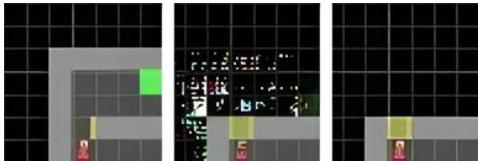
Let’s look at a concrete example. In the table below, the researchers introduce massive changes: “noise” in a Humanoid walker simulation, invisible cars in the Atari game “Freeway,” and lava in a MiniGrid environment.
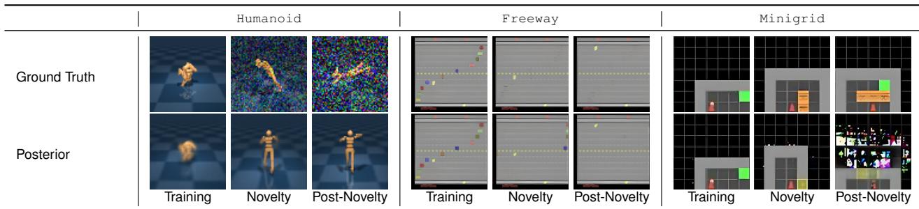
Look at the Posterior row.
- Training: The model reconstructs the image perfectly.
- Novelty Introduced: The model starts failing. In the “Freeway” example (middle column), the cars become invisible to the agent, but the model—confused by the change—hallucinates a messy, blurry reconstruction.
- Post-Novelty: The model has completely collapsed. It no longer understands the causal physics of the world.
This collapse is what we want to detect. But we want to detect it mathematically, not just by looking at blurry images.
The Method: The Novelty Detection Bound
The researchers propose a method that leverages the misalignment between the world model’s hallucinated states and the true observed states.
They introduce a concept involving “history dropout.” They ask: How much does the current image \(x_t\) contribute to our understanding compared to the history \(h_t\)?
To do this, they define a “dummy” history, \(h_0\). This acts like an agent with amnesia—it has no memory of the past.
They propose comparing two quantities using Cross Entropy (\(H\)):
- How well does the current observation (\(x_t\)) help predict the latent state if we ignore the image in the target?
- How well does it help if we keep the image in the target?
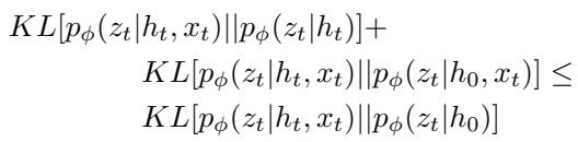
This leads to a comparison of scores:

This looks abstract, but it simplifies into a powerful inequality involving KL Divergence. The researchers derive a Novelty Threshold Bound.
The Golden Equation
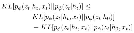
Here is the central contribution of the paper. Instead of a manual threshold, the novelty is detected when the following bound is violated:
Let’s break this down into plain English.
Left-Hand Side (LHS): \(KL[p(z_t | h_t, x_t) || p(z_t | h_t)]\).
This is the standard Bayesian Surprise. It measures how different the reality (posterior) is from the prediction (prior).
Usually, we would just set a threshold on this: “If LHS > 10, alarm!” But we don’t want to do that.
Right-Hand Side (RHS): \(KL[p(z_t | h_t, x_t) || p(z_t | h_0)] - KL[p(z_t | h_t, x_t) || p(z_t | h_0, x_t)]\).
This side acts as the Dynamic Threshold.
The first term checks how far the current state is from a “blind” guess (\(h_0\)).
The second term checks the information gain provided by the image itself.
The Intuition: Under normal conditions, your history (\(h_t\)) makes your predictions accurate. Therefore, the divergence on the Left (standard surprise) should be small. The Right side represents a “budget” of uncertainty allowed based on the complexity of the current observation.
When a novelty occurs (like invisible cars or a locked door), the model cannot reconcile the history with the new observation. The relationship flips. The standard surprise (LHS) spikes, while the model’s confidence in the observation (RHS) drops or shifts.
If LHS > RHS, we have a novelty. No manual numbers required.
Visualizing the Bound
To prove this works, the authors tracked these values over millions of training steps.
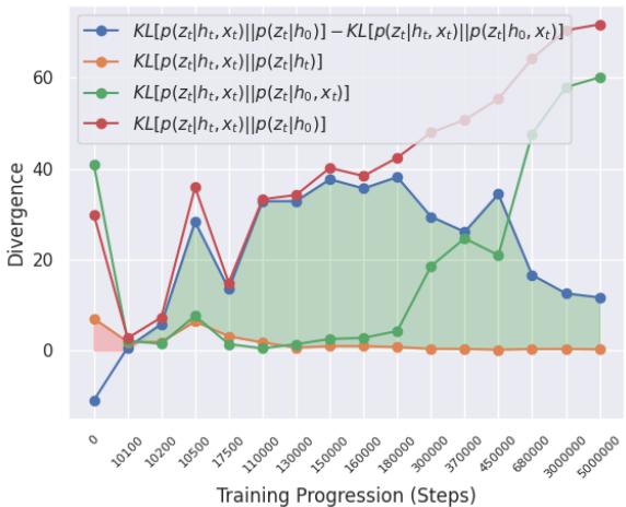
In Figure 1, look at the Blue Line. This represents the difference calculated in the bound.
- The Orange Line is the standard surprise (LHS).
- During normal training, the Orange Line stays below the Blue Line (the shaded green area). This means the bound holds: No Novelty.
- If the Orange line were to cross above the Blue line, that would trigger a detection.
This graph shows that the bound is naturally satisfied in a stationary environment, meaning the False Positive rate should be very low.
Experiments: Does it Work?
The researchers tested this on three diverse domains:
- MiniGrid: Simple 2D navigation (e.g., lava appearing, doors locking).
- Atari: Complex visual games (e.g., Boxing, Freeway, Seaquest).
- DeepMind Control (DMC): Physics-based robot control (e.g., Walker, Cheetah).
They compared their “KL Bound” method against:
- RIQN: The state-of-the-art ensemble method for RL novelty detection.
- PP-Mare: A baseline they created that looks at pixel reconstruction error (i.e., “does the image look blurry?”).
The Baseline: PP-Mare
Just for context, the PP-Mare baseline is a simpler approach that checks if the reconstructed pixels are wrong.
While simple, pixel error is often misleading. A small shift in a camera angle causes huge pixel error but isn’t necessarily “novel,” while a tiny enemy disappearing might have low pixel error but is a massive conceptual novelty.
Result 1: False Positives (The Boy Who Cried Wolf)
One of the biggest issues in anomaly detection is the False Positive Rate (FPR). If your robot stops every 5 seconds thinking it saw a ghost, it is useless.
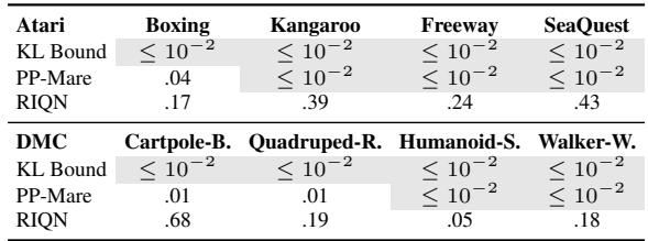
Table 2 is striking.
- RIQN: Has high false positive rates (17% to 43% in Atari!). It is overly sensitive.
- KL Bound (Ours): Consistently \(\leq 10^{-2}\) (less than 1%).
Because the KL Bound is derived from the model’s own training dynamics, it is incredibly stable in normal environments. It doesn’t “cry wolf.”
Result 2: Detection Speed and Accuracy
When novelty does happen, how fast do we catch it? We measure Average Delay Error (ADE)—how many steps pass between the novelty appearing and the alarm ringing. Lower is better.
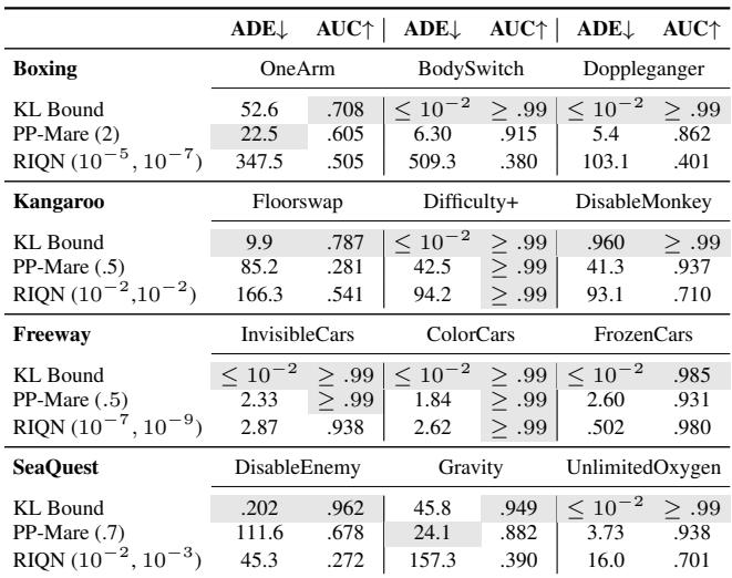
In Atari (Table 3), look at the “Freeway” environment (where cars become invisible or freeze):
- KL Bound: ADE is \(\leq 10^{-2}\). It detects it almost instantly.
- PP-Mare: Slower.
- RIQN: Competitive, but remember its high false positive rate.
In DeepMind Control (Table 4), the results are similar.
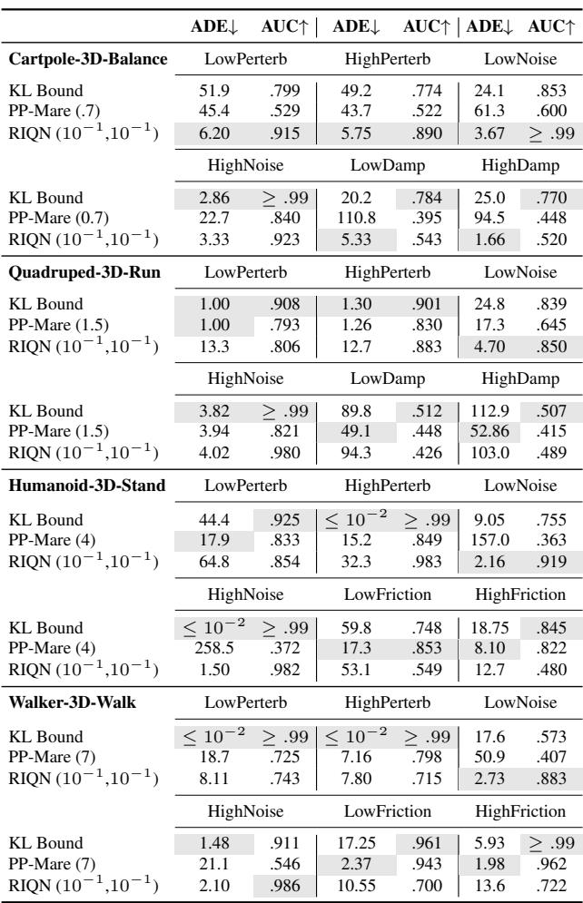
The KL Bound often achieves perfect or near-perfect detection (AUC \(\approx 0.99\)) without needing the parameter tuning that RIQN requires.
Result 3: Computational Speed
This is a blog about applying research, so we have to ask: Is it fast to run?
RIQN uses an ensemble (multiple models) and complex statistical accumulation (CUSUM). The KL Bound simply repurposes the values the World Model is already computing.
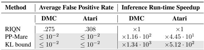
Table 6 shows the “Inference Run-time Speedup.” The KL Bound method is 1340x faster than RIQN in the DMC environment and 512x faster in Atari. This is the difference between running in real-time on a robot versus needing a supercomputer.
A Deeper Look: The “Fake Goal” Anomaly
The authors performed an interesting ablation study to show how the policy (the agent’s behavior) influences detection.
They created a “Fake Goal” environment in MiniGrid. The agent is trained to go to a goal. In the novelty setting, the goal is fake or unreachable.
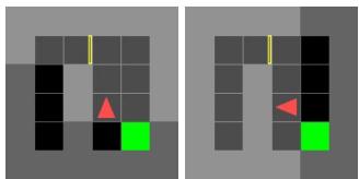
They found something fascinating: If the agent was trained efficiently, it never looked “behind” the door because it never needed to. In the novel environment, it might turn around. The World Model, having never seen the “back” of the door, flags this as a novelty.
Is seeing the back of a door a novelty? Technically, yes—it’s a transition the model hasn’t learned. But it highlights a limitation: Novelty detection relies on exploration. If your agent blindly follows a narrow path during training, anything outside that path looks like a novelty.
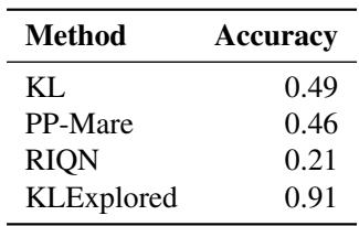
As shown in Table 8, explicitly exploring the environment (KLExplored) drastically improves the accuracy of what is flagged as a “true” novelty versus just “I haven’t looked there before.”
Generalizing to Other Architectures
The main results used DreamerV2 (RNN-based). But what about modern Transformer-based or Diffusion-based world models?
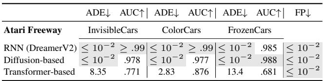
Table 7 shows that the logic holds up. Whether you use a Transformer (like IRIS) or a Diffusion model (like Diamond), the KL Bound method effectively detects novelties, though Transformers (being data-hungry) were slightly slower to react in the Freeway environment.
Conclusion and Key Takeaways
The paper “Novelty Detection in Reinforcement Learning with World Models” offers a robust solution to a critical problem in AI safety.
Here is the summary of why this matters:
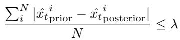
- No Magic Numbers: It eliminates the need for manual thresholds (\(\lambda\)). The bound is derived from the model’s own uncertainty dynamics.
- Using the “Surprise Gap”: It detects novelty by checking if the model relies too heavily on the current image because its history (context) no longer makes sense.
- High Precision: It drastically reduces false positives compared to state-of-the-art methods like RIQN.
- Efficiency: It is orders of magnitude faster to compute, making it viable for real-time deployment.
By repurposing the World Model—which the agent uses to plan anyway—for anomaly detection, we get a safety system almost for “free.” As we move RL out of video games and into the real world, techniques like this will be the safety net that prevents robots from failing when the world inevitably changes.