The Butterfly Effect in NLP: Disentangling Randomness in Few-Shot Learning

In the world of Machine Learning, particularly Natural Language Processing (NLP), we often chase the highest accuracy score on a benchmark. But there is a ghost in the machine: randomness.

Imagine you are training a model with very limited data—perhaps a few-shot classification task. You run the experiment and get an F1 score of 85%. You are ecstatic. But then, you change the “random seed”—a simple integer that controls how data is shuffled or how weights are initialized—and run it again. This time, the score drops to 60%.

This phenomenon is the “butterfly effect” of ML. Small, non-deterministic choices (randomness factors) can cause massive deviations in performance. This is a known problem, but new research suggests we have been diagnosing it incorrectly.

In the paper “On Sensitivity of Learning with Limited Labelled Data to the Effects of Randomness,” researchers Branislav Pecher, Ivan Srba, and Maria Bielikova argue that previous attempts to study this randomness have been flawed because they ignore the interactions between different factors.

In this deep dive, we will explore their novel methodology for disentangling these interactions and uncover which choices actually matter when training models with limited data.

The Problem: When “State-of-the-Art” is Just Luck

Learning with limited labelled data—an umbrella term covering In-Context Learning (ICL), fine-tuning, and meta-learning—is notoriously unstable.

Previous studies have identified several “randomness factors” that cause this instability:

1. Data Order: The sequence in which the model sees examples.
2. Sample Choice: Which specific examples are selected for the few-shot prompt or training set.
3. Model Initialization: The random starting weights of a neural network.
4. Data Split: How the available data is divided into training and validation sets.

The variation caused by these factors can be larger than the improvement offered by a new “state-of-the-art” architecture. This leads to a reproducibility crisis. If a model beats a benchmark only because it got a lucky random seed, have we really made progress?

The Flaw in Existing Investigations

To understand which factors hurt stability, researchers usually use one of two strategies:

1. The Random Strategy: Vary everything at once. This captures the total variance but makes it impossible to pinpoint which factor caused the drop in performance.
2. The Fixed Strategy: Fix all factors except one (e.g., fix the data order and initialization, but vary the sample choice).

The authors of this paper argue that the Fixed Strategy is misleading. Why? Because randomness factors interact.

For example, In-Context Learning (ICL) was famously believed to be highly sensitive to the order of samples in the prompt. However, later studies found this sensitivity disappeared if the samples were selected intelligently rather than randomly. This implies an interaction: the importance of “Data Order” depends heavily on “Sample Choice.” If you only study them in isolation, you get inconsistent, contradictory results.

A New Method: Investigating Randomness with Interactions

The core contribution of this paper is a rigorous mathematical framework and algorithm designed to isolate the effect of one randomness factor while statistically accounting for the others.

The method revolves around three key concepts:

1. Investigation: Varying the specific factor we want to study.
2. Mitigation: Systematically varying the other factors to average out their noise.
3. The Golden Model: A baseline representing the total variance when everything is random.

Let’s break down how this works step-by-step.

Step 1: Defining the Configurations

First, we define the set of all randomness factors (RF). Let’s say we want to investigate factor \(i\) (e.g., Data Order). We need to distinguish between the factor we are looking at and the “background” factors we need to mitigate.

The authors define a Mitigated Factor Configuration (\(MFC_i\)). This is the set of all possible combinations of the other factors.

In this equation:

• \(\mathbb{C}_i\) is the set of configurations for the factor we are investigating.
• The equation represents the cross-product of all other configuration sets (\(\mathbb{C}_1\) through \(\mathbb{C}_K\), excluding \(i\)).

Step 2: The Investigation Loop

To analyze factor \(i\), the algorithm performs a nested loop.

1. It fixes the “background” factors to a specific configuration (\(m\)).
2. It then varies the investigated factor \(n\) across all its possibilities.
3. It measures the model’s performance (\(r_{m,n}\)).

This generates a matrix of results, which is best visualized in the table below:

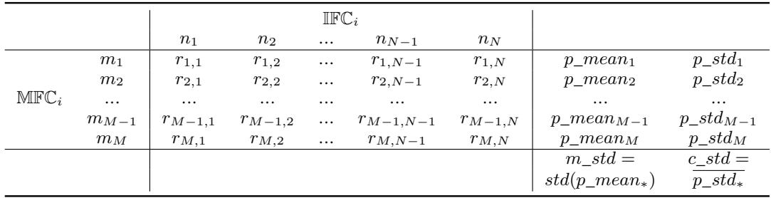
Understanding the Table:

• Columns (\(n_1, n_2...\)): These are the different states of the factor you are studying (e.g., different permutations of data order).
• Rows (\(m_1, m_2...\)): These are different “fixed” states of the rest of the universe (e.g., a specific data split and model initialization).

Step 3: Calculating Contributed vs. Mitigated Deviation

This is where the math gets clever. The authors calculate two distinct types of standard deviation to separate the signal from the noise.

1. Contributed Standard Deviation (\(c\_std\)): Look at a single row in the table above. The variation in numbers across that row (\(p\_std_m\)) tells us how much the performance changes due to the investigated factor when everything else is held constant. The authors calculate this for every row (every background configuration) and average them. This represents the “pure” effect of the factor \(i\).

2. Mitigated Standard Deviation (\(m\_std\)): Look at the column \(p\_mean\) on the right. Each value here is the average performance for a specific background configuration. If we take the standard deviation of these means, we get the \(m\_std\). This number tells us how much the performance swings due to the interaction of all the other background factors.

Step 4: The Importance Score

Finally, to determine if a factor actually matters, it is compared against a Golden Model. The Golden Model is trained by varying all factors simultaneously. Its standard deviation (\(gm\_std\)) represents the “total chaos” or total instability of the system.

The Importance Score is calculated as:

• Interpretation: If the score is greater than 0, the factor is significant. It contributes more to the variance than all other factors combined. If it is low or negative, the instability is actually coming from the interactions of other factors, not the one you are investigating.

Experimental Results: Busting Myths

The authors applied this method to three major paradigms: In-Context Learning (using models like Flan-T5, LLaMA-2, Mistral, Zephyr), Fine-Tuning (BERT, RoBERTa), and Meta-Learning. They tested across 7 datasets including GLUE tasks and multi-class classification tasks like AG News and DB-Pedia.

Here is what they found when they disentangled the interactions.

1. The “Data Order” Myth in In-Context Learning

A widely held belief in the NLP community is that In-Context Learning (ICL) is extremely sensitive to the order of examples in the prompt.

However, when the authors applied their method, they found that Data Order is not consistently important for ICL on binary classification tasks. When interactions were properly accounted for, the “instability” attributed to order was actually largely driven by Sample Choice (which specific examples were picked).

The chart below summarizes the Importance Scores across different models and datasets.

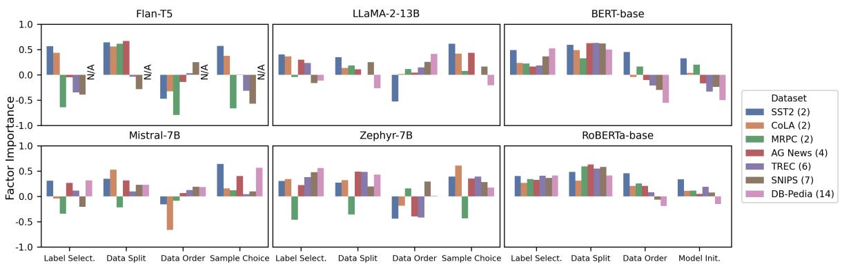
Key Takeaways from Figure 1:

• Sample Choice (Far Right): Notice the generally high positive bars for Sample Choice in the ICL models (top rows). This is the dominant factor.
• Data Order (Second from Right): For binary datasets (like SST2, colored in lighter shades), the importance is often negative or low. However, look at the darker bars (representing multi-class datasets like DB-Pedia). As the number of classes increases, Data Order does become important again.
• Fine-Tuning (Bottom Rows): For BERT and RoBERTa, the story is different. They are highly sensitive to Label Selection and Data Split, but less so to Model Initialization (except for binary tasks).

2. Systematic Choices: Number of Shots and Classes

The authors hypothesized that “systematic choices”—decisions we make consciously, like how many shots to use or how many classes to predict—alter the landscape of randomness.

Does adding more shots stabilize the model?

We often assume that providing more examples (10-shot vs. 2-shot) reduces variance. The results show a nuance:

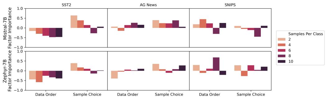
In Figure 2, we see:

• Sample Choice (Right Column): As the number of shots (samples per class) increases (moving from light orange to black bars), the importance of Sample Choice decreases. This makes sense—choosing 10 bad examples is statistically harder than choosing 1 bad example.
• Data Order (Left Column): Surprisingly, increasing the number of shots does not consistently reduce sensitivity to Data Order. The model remains just as confused by a bad ordering of 10 examples as it does by 2.

3. The Impact of Prompt Format

Perhaps the most striking finding involves the prompt template itself. The researchers tested an “Optimized” prompt against three “Minimal” prompt formats (e.g., just “Sentiment: [Output]” vs. “Determine the sentiment of the sentence…”).

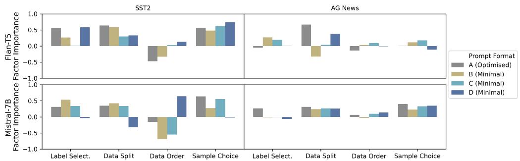
Observations from Figure 3:

• Sensitivity to Format: Look at the Flan-T5 model (left side). The importance scores swing wildly depending on the format (A, B, C, D). Minimal formats often spiked the sensitivity to randomness.
• Model Size Matters: The larger model, Mistral-7B (right side), is much more robust. The bars are relatively stable across different prompt formats. This suggests that larger instruction-tuned models have internalized the task definition better and are less reliant on the specific phrasing of the prompt to stabilize their randomness.

4. Meta-Learning Findings

Finally, the authors investigated Meta-Learning approaches (like MAML and Reptile).

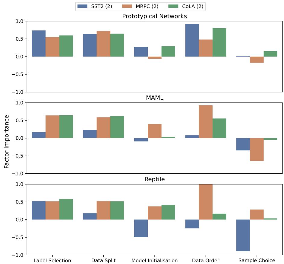
For Meta-Learning on binary datasets, Data Order (specifically the order of tasks/batches) reigns supreme. It is consistently the most important factor, often reaching an importance score of 1.0 (contributing nearly all the deviation). This is a crucial insight for researchers training meta-learning algorithms: how you shuffle your tasks matters more than almost anything else.

Conclusion and Implications

This research serves as a critical “reality check” for the NLP community. It highlights that the instability we observe in few-shot learning is not a monolith—it is a complex web of interacting factors.

Key Takeaways for Students and Practitioners:

1. Don’t Trust Simple Standard Deviations: If you read a paper that claims “Method X is robust to random seeds,” check how they tested it. Did they vary only the seed while fixing the data split? If so, they might be underestimating the true variance.
2. Prioritize Sample Choice in ICL: If you are building an application using In-Context Learning (like GPT-4), spending time on how you select your few-shot examples (retrieval-based selection) yields better stability returns than worrying about their order (unless you have many classes).
3. Context Matters: A randomness factor that is fatal for a binary classification task might be negligible for a multi-class task, and vice versa.
4. Use the Method: The algorithm proposed by Pecher et al. (Investigate-Mitigate-Compare) provides a blueprint for honest, reproducible reporting of model stability.

As models grow larger and opaque, understanding the “ghosts” of randomness becomes more important, not less. By dissecting these interactions, we move from alchemy—hoping for a lucky seed—to chemistry, where we understand the properties of our elements.