](https://deep-paper.org/en/paper/2402.13593/images/cover.png)
Beyond Cut and Paste: Editing LLMs with Knowledge Graphs
Imagine you are reading a biography of LeBron James generated by a Large Language Model (LLM). The model correctly states, “LeBron James plays for the Los Angeles Lakers.” But when you ask, “Does LeBron James work in Los Angeles?” the model hesitates or, worse, confidently replies, “No, he works in Miami.”
This inconsistency highlights a critical flaw in current AI systems. LLMs store vast amounts of world knowledge, but that knowledge can become outdated or remain factually incorrect. While we have methods to “edit” specific facts—like updating a database entry—LLMs struggle with the ripple effects of those edits. Changing a team affiliation should logically change the city of employment, the teammates, and the home stadium.
In this post, we will deep dive into a research paper titled “Knowledge Graph Enhanced Large Language Model Editing”, which introduces a novel method called GLAME. This method doesn’t just patch a single fact; it uses Knowledge Graphs (KGs) to understand and update the web of connections surrounding that fact, ensuring the model remains consistent and capable of reasoning with the new information.
The Problem: The Ripple Effect
Model editing is the process of altering an LLM’s parameters to correct specific knowledge without retraining the entire model (which is prohibitively expensive). Existing methods like ROME (Rank-One Model Editing) and MEMIT have been successful at updating singular facts, such as changing \((s, r, o)\) to \((s, r, o^*)\).
However, knowledge is rarely isolated. It is interconnected.
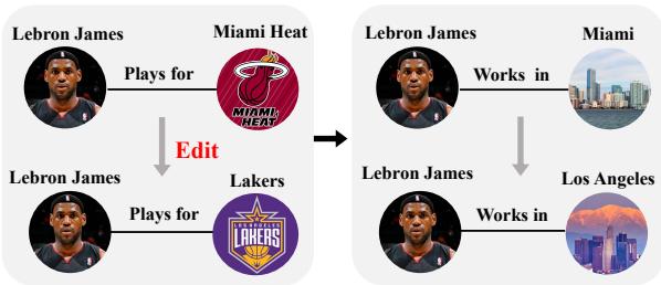
As shown in Figure 1 above, if we update the fact that LeBron James plays for the Miami Heat to the Los Angeles Lakers, the model must also infer that he now works in Los Angeles. If the model updates the explicit fact but fails to update the associated implications, the model becomes internally inconsistent. This failure limits the generalization ability of the post-edit LLM.
The researchers argue that the “black-box” nature of LLMs makes it hard to detect these associations internally. Therefore, they propose bringing in an external map: a Knowledge Graph.
Background: How Model Editing Works
To understand GLAME, we first need to understand the foundation it builds upon: Rank-One Model Editing (ROME).
The ROME method operates on the hypothesis that Feed-Forward Networks (FFNs) within Transformer layers act as Key-Value Memories. In this conceptual framework, a specific subject (like “LeBron James”) acts as a key, and the output of the layer acts as the value (attributes like “plays for Lakers”).
Mathematically, the output of an FFN layer \(l\) for the \(i\)-th token is described as:
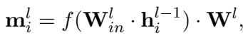
Here, \(\mathbf{h}_i^{l-1}\) is the input from the previous layer. The first part of the operation creates a “key” (\(\mathbf{k}\)), and the second weight matrix \(\mathbf{W}^l\) transforms it into a “value” (\(\mathbf{m}\)).
The Optimization Goal
When editing a model, the goal is to find a new weight matrix \(\hat{\mathbf{W}}\) that satisfies a specific constraint: when the model sees the key for the subject (\(\mathbf{k}_*\)), it should output a specific target vector (\(\mathbf{m}_*\)) that represents the new fact. At the same time, we want to change the weights as little as possible to avoid breaking other knowledge.
This is formulated as a constrained least-squares problem:
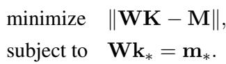
Here, \(\mathbf{K}\) and \(\mathbf{M}\) represent all the other knowledge we want to preserve, while the constraint \(\mathbf{Wk}_* = \mathbf{m}_*\) ensures our specific edit works.
ROME provides a closed-form solution to calculate the new weights:
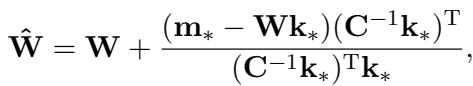
In this equation, \(\mathbf{C}\) is a covariance matrix of keys pre-calculated from a text corpus (like Wikipedia).
The Limitation of ROME: ROME calculates the target vector \(\mathbf{m}_*\) by optimizing solely for the specific target fact (LeBron -> Lakers). It doesn’t explicitly look at the neighbors (Lakers -> Los Angeles). This is where GLAME steps in.
The Core Method: GLAME
GLAME (Graphs for LArge language Model Editing) enhances the editing process by explicitly modeling the “ripple effects” using a Knowledge Graph. The architecture is split into two main modules:
- Knowledge Graph Augmentation (KGA): Finds the associated knowledge.
- Graph-based Knowledge Edit (GKE): Injects this structure into the model.
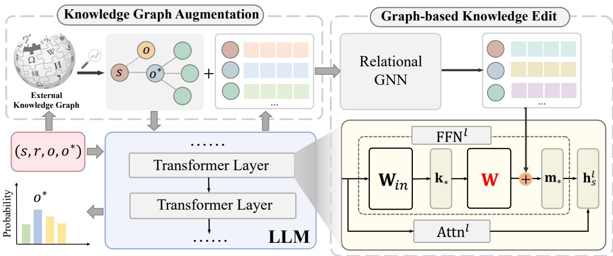
Let’s break down the architecture illustrated in Figure 2.
Module 1: Knowledge Graph Augmentation (KGA)
When the system receives an edit request \(e = (s, r, o, o^*)\), it doesn’t just look at the text. It queries an external Knowledge Graph (like Wikidata) to find the new object \(o^*\) and its neighbors.
For example, if \(o^*\) is “Los Angeles Lakers,” the KGA module might pull in triples like (Lakers, located in, Los Angeles) or (Lakers, part of, NBA). It constructs a subgraph containing these new high-order relationships.
But raw graph data isn’t enough; the LLM needs to “understand” these entities in its own language. The researchers initialize the representation of the entities in this subgraph using the LLM itself. They feed the text of the entities into the LLM and extract the hidden states from the early layers:
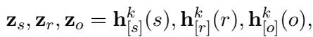
By using the hidden states \(\mathbf{h}_{[s]}^k\) from the early layers (layer \(k\)), they obtain a vector representation that aligns with the LLM’s internal embedding space.
Module 2: Graph-based Knowledge Edit (GKE)
Now that we have a subgraph representing the new context, we need to encode it. The researchers employ a Relational Graph Neural Network (RGNN).
The RGNN aggregates information from the neighbors to update the representation of the subject \(s\). This effectively “teaches” the subject vector about its new connections.
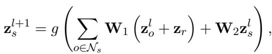
In this equation:
- \(\mathcal{N}_s\) is the set of neighbors.
- \(\mathbf{W}_1\) and \(\mathbf{W}_2\) are learnable weights of the GNN.
- The function aggregates the neighbor vectors \(\mathbf{z}_o\) and relation vectors \(\mathbf{z}_r\) to update the subject \(\mathbf{z}_s\).
This process creates a “context-aware” representation of the subject, denoted as \(\mathbf{z}_s^n\).
Injecting the Knowledge
Here is the clever part. Instead of optimizing a random vector to be the target \(\mathbf{m}_*\), GLAME defines the target vector as the original memory of the subject shifted by the graph encoding:
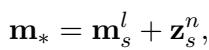
This equation says: “The new memory for this subject should be its old memory (\(\mathbf{m}_s^l\)) plus the information gained from the knowledge graph (\(\mathbf{z}_s^n\)).”
Optimization
GLAME does not update the LLM parameters directly during the training phase. Instead, it trains the RGNN parameters to produce the perfect \(\mathbf{m}_*\).
The loss function has two parts. First, the Prediction Loss ensures the modified memory actually causes the model to predict the new object \(o^*\):
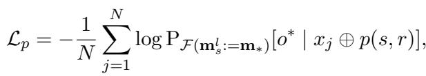
Second, a Regularization Loss (KL Divergence) ensures that the subject’s general representation remains stable (e.g., “LeBron is a basketball player” shouldn’t change, even if his team does).
The total loss combines these two:
Once the RGNN is trained to minimize this loss, we have our optimal \(\mathbf{m}_*\). We also calculate the key vector \(\mathbf{k}_*\) using the standard method:
Finally, with the optimal \(\mathbf{m}_*\) (enhanced by the graph) and \(\mathbf{k}_*\), GLAME uses the exact same closed-form update equation as ROME (see Equation 3) to update the LLM’s weights.
Experiments & Results
The researchers evaluated GLAME on GPT-2 XL (1.5B parameters) and GPT-J (6B parameters). They used three datasets:
- COUNTERFACT: The standard benchmark for single edits.
- COUNTERFACTPLUS: A harder dataset requiring reasoning.
- MQUAKE: A dataset specifically for multi-hop questions.
Metrics Explained
- Efficacy Score: Did the edit work? (Does it say “Lakers”?)
- Paraphrase Score: Does it work if I rephrase the question?
- Neighborhood Score: Did we break unrelated facts?
- Portability Score: Can the model reason using the new fact? (This is the most critical metric for GLAME).
Performance Comparison
Table 1 below shows the main results.
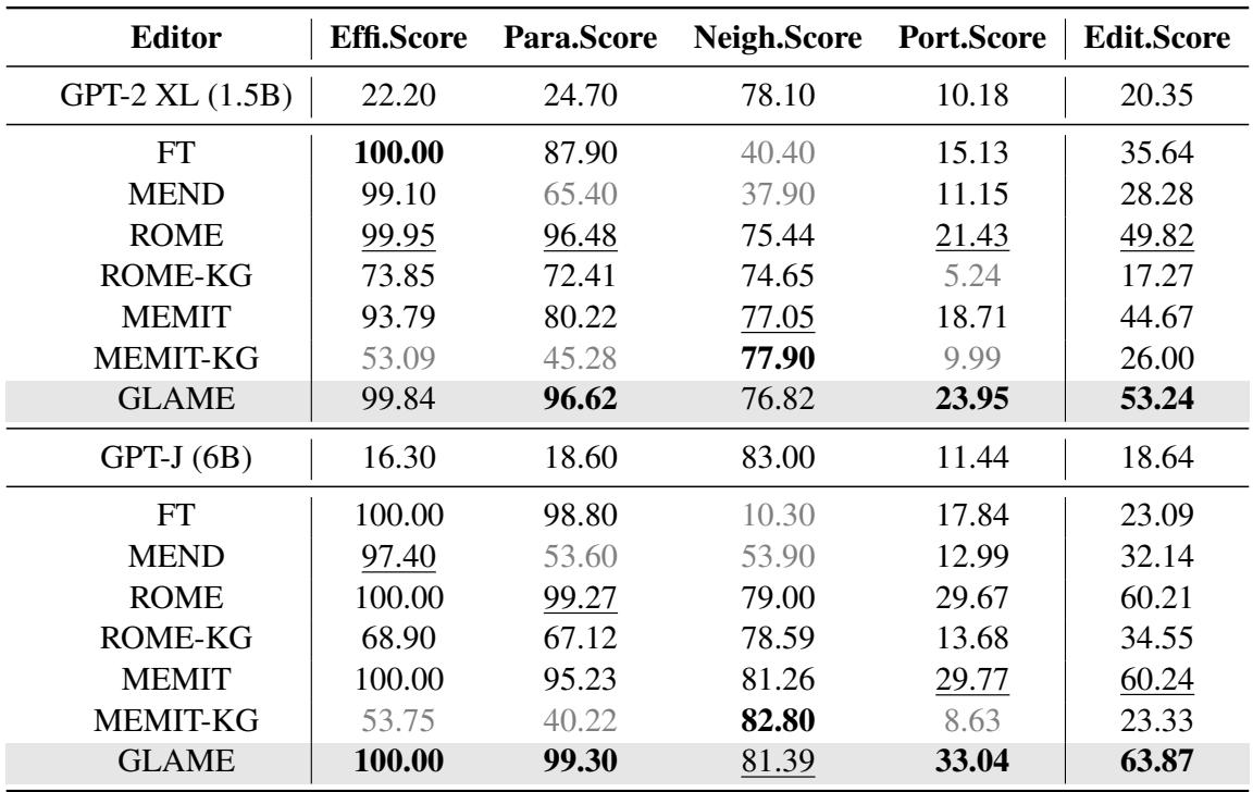
Key Takeaways:
- Portability is King: GLAME significantly outperforms all baselines in the Portability Score. For GPT-J, GLAME achieves a score of 33.04%, compared to ROME’s 29.67% and MEMIT’s 29.77%. This proves that including the knowledge graph helps the model reason about the consequences of the edit.
- High Editing Score: GLAME achieves the highest overall “Editing Score” (harmonic mean of metrics) on both models.
- The Baseline Failure: Look at “ROME-KG” and “MEMIT-KG.” These were baselines where the authors tried to simply force-feed the graph triples into ROME/MEMIT as text edits. The performance dropped drastically. This shows that simply having the data isn’t enough; you need the structured integration provided by the RGNN in GLAME.
Ablation Studies: Do we need the Graph?
The authors stripped down GLAME to see which parts mattered.
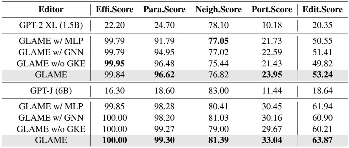
- GLAME w/ MLP: Replaced the Graph Neural Network with a simple MLP (ignoring the graph structure). Performance dropped.
- GLAME w/o GKE: Removed the graph module entirely (essentially reverting to ROME). Performance dropped.
- Conclusion: The structural relationships processed by the GNN are essential for capturing the ripple effects.
Sensitivity Analysis
How complex should the knowledge graph be?
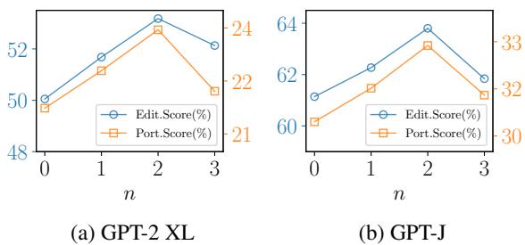
Figure 3 shows the effect of the subgraph order (\(n\)). \(n=1\) means direct neighbors, \(n=2\) means neighbors of neighbors. The results show that \(n=2\) is the sweet spot. Going deeper (\(n=3\)) introduces noise and hurts performance.
Similarly, looking at the number of neighbors (\(m\)):
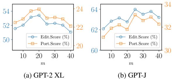
Figure 4 suggests that sampling around 20-25 neighbors is optimal. Too few, and you miss context; too many, and the signal gets drowned out by noise.
MQUAKE Results: The Ultimate Reasoning Test
Finally, the authors tested on MQUAKE, a dataset designed for multi-hop reasoning (e.g., “Who is the head of state of the country from which the music genre associated with [Artist] originated?”).
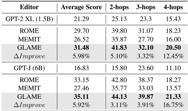
GLAME outperforms ROME and MEMIT across 2-hop, 3-hop, and 4-hop questions. The gap widens at 4-hops, suggesting that for highly complex reasoning chains, the structured knowledge injection is vastly superior to simple fact editing.
Conclusion and Implications
The “GLAME” paper presents a compelling step forward in making Large Language Models more reliable and maintainable. By acknowledging that facts do not exist in a vacuum, the researchers have moved beyond simple “find and replace” editing.
The key takeaways are:
- Context Matters: Editing a single fact requires updating the web of associated knowledge to maintain consistency.
- Graphs are Powerful: External Knowledge Graphs provide the structured context that LLMs struggle to infer on their own.
- Structured Injection: Simply training on graph text isn’t efficient. Using a GNN to encode the graph and modifying the internal memory vectors is a much more effective strategy.
As LLMs become more integrated into critical applications, the ability to accurately update their knowledge bases without expensive retraining will be essential. GLAME demonstrates that the bridge between symbolic AI (Knowledge Graphs) and neural AI (LLMs) is a promising path toward smarter, more adaptable models.