Beyond Neurons: Finding and Fixing the Interpretable Circuits Inside LLMs

Language models like GPT-4 can write poetry, code, and convincing essays. But how do they do it? Ask an AI researcher, and you might get a complicated chart full of “neurons” and “attention heads.” That’s like trying to understand a novel by inspecting the letters—it tells you something, but not much about the story. Each neuron is polysemantic, playing dozens of roles at once. This makes it hard to connect what the model does to how it does it, creating major challenges for safety, reliability, and bias control.

What if we could find the equivalent of words or sentences inside these models—distinct concepts we can name, like “detect plural noun” or “identify a date”? And what if we could trace how these concepts interact to form the reasoning that drives a model’s predictions?

A new research paper, “Sparse Feature Circuits: Discovering and Editing Interpretable Causal Graphs in Language Models,” introduces a method to do exactly that. The authors present a powerful technique for automatically discovering sparse feature circuits—causal graphs that explain model behaviors in terms of human-understandable semantic units instead of opaque neurons.

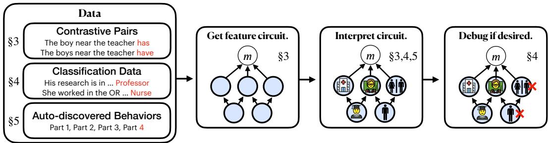
Figure 1: Overview of the sparse feature circuit approach—from data to interpretable causal graphs.

This breakthrough isn’t just about peeking inside language models—it’s about changing them responsibly. Using these circuits, the authors show how to surgically edit a model’s behavior, such as removing gender bias from a classifier, without special debiasing data. In this post, we’ll unpack how these circuits are built and why they matter.

Overview

We’ll explore five key ideas from the paper:

1. The foundations: Sparse Autoencoders (SAEs) for discovering concepts, and Causal Tracing for measuring their influence.
2. How the authors assemble sparse feature circuits from these ingredients.
3. What these circuits reveal about linguistic reasoning.
4. How the SHIFT technique edits models to remove spurious signals.
5. How the entire process can scale up to explain thousands of behaviors automatically.

The Building Blocks: Concepts and Causality

To build interpretable circuits, we first need a way to extract meaningful features—and a way to measure how much those features causally affect the model’s predictions. The paper combines two complementary ideas to achieve both.

Finding Interpretable Features with Sparse Autoencoders (SAEs)

Inside a language model, each activation is a vector in a high-dimensional space. A single neuron corresponds to one direction in this space—often an unintelligible jumble of unrelated patterns. Sparse Autoencoders (SAEs) replace those neurons with interpretable directions.

An SAE learns a dictionary of features that can reconstruct model activations efficiently, while enforcing sparsity so that only a few features activate per input. This tends to yield monosemantic features—clean representations of distinct concepts such as “female pronoun,” “number token,” or “noun phrase boundary.”

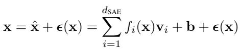
Equation 1: Sparse Autoencoder decomposition of activations.

Formally, the SAE reconstructs an activation vector \( \mathbf{x} \) as a sparse sum of feature activations \( f_i(\mathbf{x}) \) multiplied by feature vectors \( \mathbf{v}_i \), plus a small error term \( \epsilon(\mathbf{x}) \). The authors keep this error term, treating it as a placeholder for unexplained contributions. By training SAEs across all major components of models like Pythia-70M and Gemma-2-2B, they construct large, interpretable dictionaries of model features—our raw material for circuits.

Finding What Matters with Causal Tracing

Knowing what features represent is only half the battle. To understand how they influence the model’s output, the authors use causal mediation analysis, which measures the indirect effect (IE) of a component inside the model.

Equation 2: Computing the indirect causal effect.

For example, consider the sentences:

• Clean: “The teacher is…”
• Patch: “The teachers are…”

By patching activations from the plural example into the clean one, we can observe how strongly a particular feature (like one that detects plurality) drives the model’s verdict between “is” and “are.”

Because evaluating every component precisely is too expensive, the paper develops fast linear approximations. The simplest, attribution patching, uses gradients of the output with respect to each activation:

Equation 3: Attribution patching for causal effect estimation.

A more accurate method, integrated gradients, averages those gradients along a path between clean and patched activations:

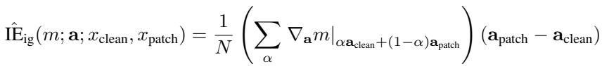
Equation 4: Integrated gradients improve accuracy for complex components.

With interpretable features (the what) and causal effects (the how much), we’re ready to map entire causal circuits.

The Core Method: Discovering Sparse Feature Circuits

Instead of viewing the model as a web of neurons, the authors treat it as a graph of features. Each node represents a specific SAE feature or its error term at a particular token position. Using causal tracing, they identify which nodes and edges exert meaningful influence on the output.

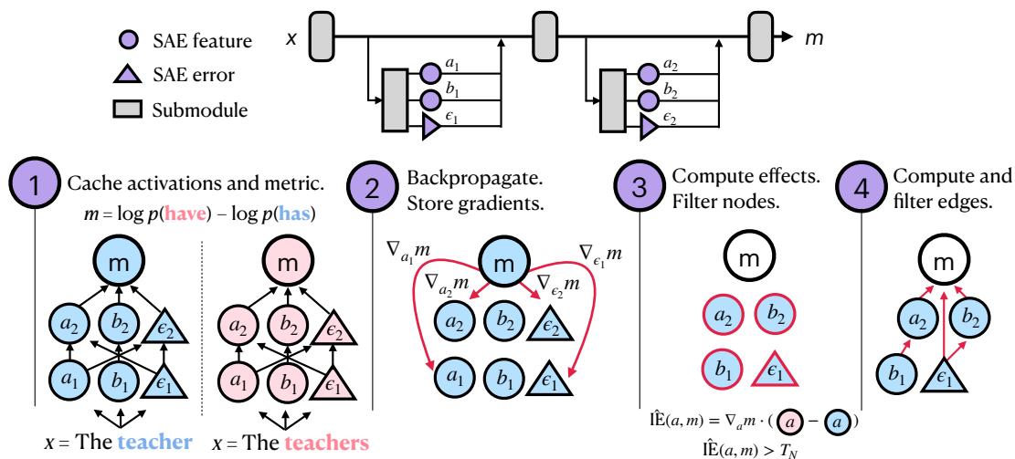
Figure 2: Four-step procedure for circuit discovery using causal tracing.

The process unfolds as:

1. Cache Activations and Gradients: Run the model on relevant data (like contrastive input pairs) while collecting all feature activations and gradients.
2. Backpropagate Effects: Compute gradients of the chosen metric (e.g., difference in log-probabilities between “has” and “have”).
3. Filter Nodes: Estimate each node’s indirect effect using the linear approximations. Discard low-impact nodes to get a sparse, focused set.
4. Filter Edges: Compute causal effects between nodes to identify which connections truly matter.

The result is a concise directed graph—a sparse feature circuit—that captures how distinct, interpretable concepts cooperate to drive the model’s behavior.

Testing the Circuits: Subject–Verb Agreement

To validate the approach, the authors test it on subject–verb agreement, a classic linguistic phenomenon with varying complexity.

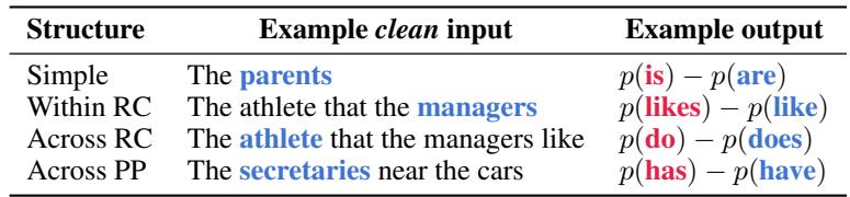
Table 1: Subject–verb agreement structures used for circuit discovery.

Evaluation focuses on three dimensions:

1. Interpretability: Human annotators rate SAE features from circuits as far more understandable than random features or raw neurons.
2. Faithfulness: How well does a circuit replicate the model’s results if everything outside it is ablated?
3. Completeness: Does ablating only the circuit destroy the model’s performance?

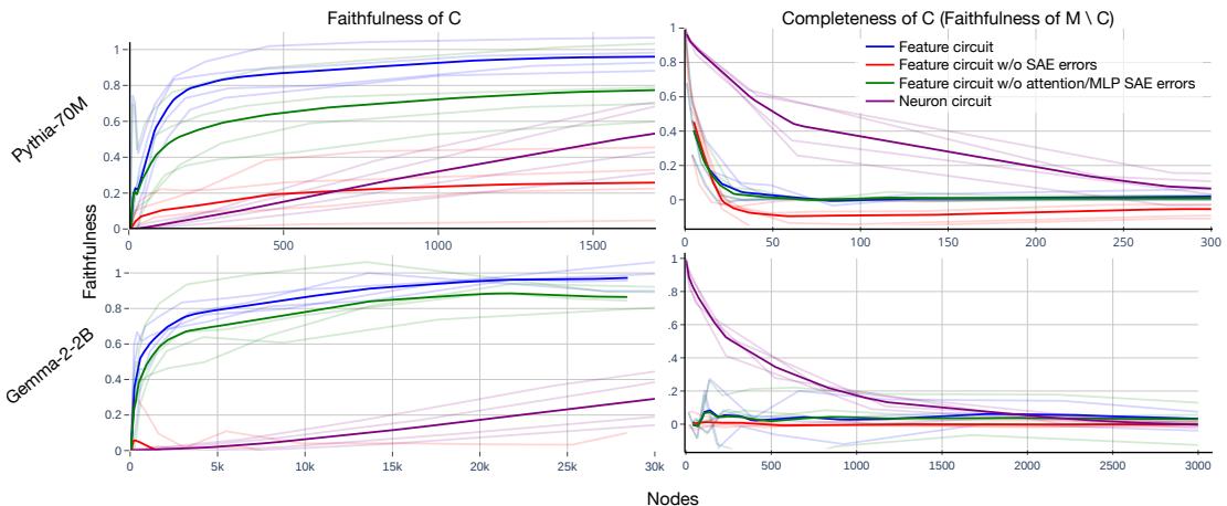
Figure 3: Feature circuits explain model behavior more efficiently and completely than neuron-level circuits.

The result: small feature circuits capture most of the model’s reasoning. For Pythia-70M, fewer than 100 features reproduce the behavior as well as 1,500 neurons. Ablating just those features wipes out the model’s grammatical ability—evidence that the discovered circuit is both faithful and complete.

Case Study: Agreement Across a Relative Clause

Consider the challenge: “The girl that the teacher sees has” vs. “The girls that the teacher sees have.” The model must ignore the distractor “teacher” and link “girls” to “have.”

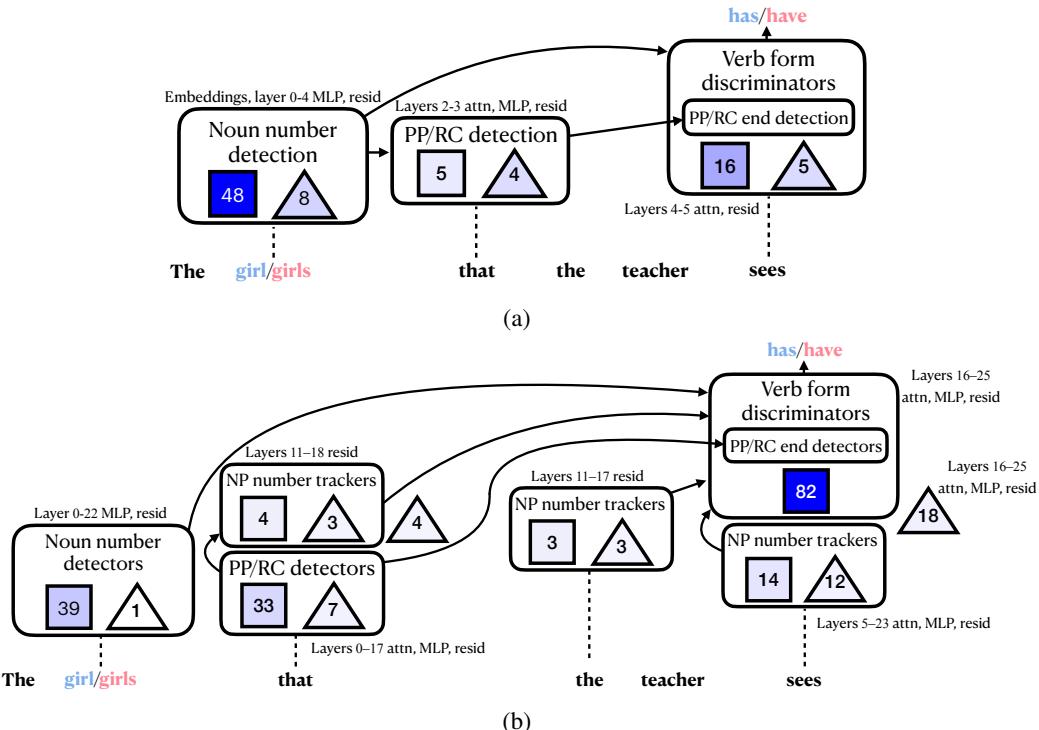
Figure 4: Circuits for subject–verb agreement across a relative clause in Pythia and Gemma.

The resulting circuits reveal clear, interpretable reasoning:

1. Noun Number Detection: Early features fire on the subject (“girl”/“girls”) to detect singular vs. plural.
2. Boundary Detection: Features recognize relative clause markers like “that,” signaling the start of a distractor phrase.
3. Information Propagation: Subject-number information moves forward through layers. Gemma-2-2B maintains dedicated noun phrase number trackers that stay active throughout the phrase.
4. Verb Form Selection: Near the output, verb-inflection features apply the captured number information to choose “has” or “have.”

These steps outline a human-readable “algorithm” for language understanding inside the model.

Editing Bias with SHIFT

Interpretability becomes most powerful when we can use it to improve models. The authors demonstrate this with Sparse Human-interpretable Feature Trimming (SHIFT), a technique for removing unintended signals from classifiers.

The Problem

Trained classifiers often rely on spurious cues—like gender correlating with profession. Prior debiasing methods need special labeled datasets to isolate these signals. SHIFT works without any disambiguating data, relying solely on interpretability and human judgment.

The Method

1. Discover the classifier’s feature circuit using the sparse-feature method.
2. Inspect each feature and label it as task-relevant or spurious.
3. Ablate spurious features (e.g., those activating on gendered words).
4. Optionally retrain the final classification layer using the same biased data.

The Test: Bias in Bios

The authors use the Bias in Bios (BiB) dataset—biographies labeled with both profession and gender. The tricky ambiguous set contains only male professors and female nurses, so gender perfectly predicts profession. SHIFT must rebuild a classifier that learns profession without access to gender.

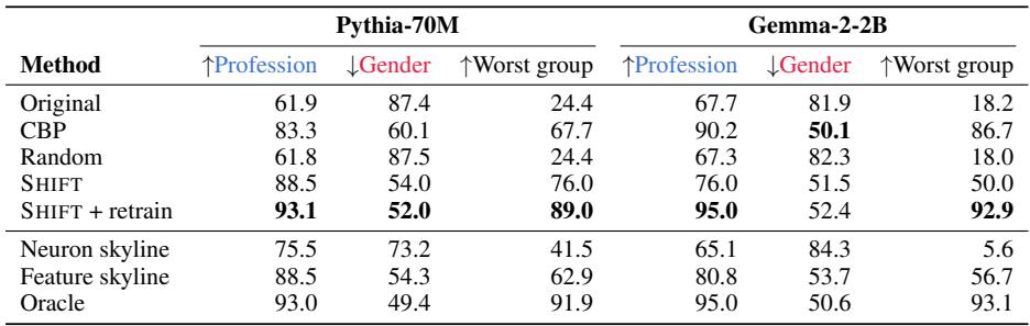
Table 2: SHIFT removes gender bias while preserving or improving performance.

Results speak volumes. Using SHIFT on Pythia-70M:

• Original classifier accuracy on profession: 61.9%
• After SHIFT + retraining: 93.1%, nearly matching an oracle model trained on unbiased data.
• Gender prediction accuracy drops from 87.4% to 52.0%—essentially removing bias.

When applied to neurons instead of SAE features, this success vanishes: neurons mix multiple meanings, so ablating them destroys useful information. SHIFT works because sparse features are disentangled, making causal editing precise and meaningful.

Scaling Up: Automated Circuit Discovery

So far, we’ve manually selected tasks. But language models exhibit thousands of subtle, emergent behaviors. To explore them all, the researchers build a fully automated pipeline for unsupervised behavior discovery.

1. Discover Behaviors: Run the model on a huge corpus (The Pile), extract internal representations or gradients, and cluster them—grouping contexts that trigger similar mechanisms.
2. Discover Circuits: Apply the sparse feature circuit method to each cluster automatically.

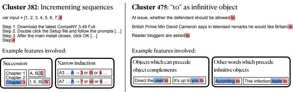
Figure 5: Automatically discovered circuits for number succession and infinitival “to”.

Examples include:

• Incrementing sequences: The model combines broad “succession” features with “narrow induction” features that recognize patterns like A3 ... A → 4.
• Infinitive objects: Separate mechanisms detect verbs that take “to” complements and direct objects that precede them.

This automated system produces thousands of interpretable circuits. You can explore them interactively at feature-circuits.xyz.

Conclusion

Sparse Feature Circuits mark a milestone for mechanistic interpretability. By shifting focus from opaque neurons to clean, human-interpretable sparse features, the authors achieve:

• Interpretability: Clear causal graphs of meaningful concepts.
• Faithfulness: Circuits that replicate model behavior accurately.
• Actionability: Methods like SHIFT for precise, ethical model editing.
• Scalability: Automated pipelines revealing thousands of internal mechanisms.

The approach transforms interpretability from a passive tool into an active one—allowing us not just to observe how models think, but to shape that thinking responsibly. Future progress will depend on developing even better sparse autoencoders and systematic evaluation methods. But the vision is clear: a world where AI is transparent, editable, and aligned—because we finally understand its circuits.