LLMs Judging LLMs: How to Rank Texts Efficiently with a Product of Experts Framework

As Large Language Models (LLMs) continue to dominate the landscape of Natural Language Processing, a secondary, equally difficult problem has emerged: How do we evaluate them?

When an LLM generates a summary, a story, or a line of dialogue, there is rarely a single “correct” answer. Traditional metrics like BLEU or ROUGE, which rely on word overlap with a reference text, often fail to capture nuances like coherence, creativity, or helpfulness. This has led to the rise of LLM-as-a-judge, where we use a stronger model (like GPT-4 or Llama-2-Chat) to grade the outputs of other models.

Currently, the gold standard for this evaluation is pairwise comparison. Instead of asking a model to “Rate this text 1 to 10” (which is notoriously inconsistent), we ask, “Which text is better: A or B?”

However, there is a catch. If you have 100 candidate responses to rank, comparing every single pair requires nearly 10,000 API calls. The cost scales quadratically (\(O(N^2)\)). For large-scale benchmarks, this is prohibitively expensive and slow.

In this post, we will dive deep into a research paper by Liusie et al. from the University of Cambridge, which proposes a mathematical framework called Product of Experts (PoE). This method allows us to rank texts accurately using only a tiny fraction of the total possible comparisons—saving computation while maintaining high correlation with human judgment.

The Intuition: Comparisons as “Experts”

To understand the solution, we first need to refine how we look at the problem.

In a standard ranking scenario, you have a set of items (texts) with underlying “true” scores. When an LLM compares Text A and Text B, it makes a decision. Traditionally, we treat this as a binary outcome: A wins, or B wins. We then plug these wins and losses into algorithms like the Bradley-Terry model (similar to the ELO system in chess) to estimate the scores.

But LLMs give us more than just a binary decision. They provide probabilities. An LLM might say, “I am 90% sure A is better than B,” or “I am 51% sure A is better.” Traditional methods often throw this rich uncertainty information away, converting it into a hard “Win” or “Loss.”

The authors of this paper propose a different view: Treat every pairwise comparison as an independent “Expert.”

Imagine a room full of experts. One expert looks at Text A and Text B and gives you a probability distribution of how much better A is than B. Another expert looks at Text B and Text C. The Product of Experts framework mathematically combines all these independent opinions to find the most likely scores for all texts simultaneously.

The Mathematical Foundation

Formally, let’s say we have \(N\) candidate texts. We want to find their scores, denoted as \(s_{1:N}\). We have a set of \(K\) pairwise comparisons, \(\mathcal{C}_{1:K}\).

The probability of a specific set of scores, given our comparisons, can be modeled by multiplying the probabilities given by each individual comparison (expert). The goal is to find the scores that maximize this probability:

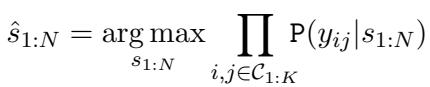
Here, \(\mathbb{P}(y_{ij} | s_{1:N})\) is the likelihood of the observed outcome given the scores.

In the Product of Experts (PoE) view, we generalize this. We aren’t just looking at binary outcomes (\(y_{ij}\)), but rather the information provided by the comparison \(C_k\) regarding the difference in scores between text \(i\) and text \(j\).

The probability of the scores given the comparisons is defined as the product of the individual experts, normalized by a constant \(Z\):

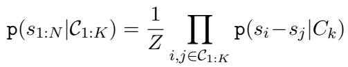
This equation is the backbone of the framework. It says: “The likelihood of these scores being true is the product of what every single comparison tells us about the score differences.”

Two Types of Experts

The framework is flexible—you can plug in different mathematical models for your “experts.” The paper explores two main variants.

1. The Soft Bradley-Terry Expert

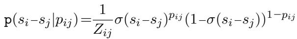
The traditional Bradley-Terry model uses a sigmoid function (\(\sigma\)) to model the probability that Text \(i\) beats Text \(j\) based on their score difference (\(s_i - s_j\)).

The authors extend this to handle soft probabilities (\(p_{ij}\)) output by the LLM. If the LLM predicts Text \(i\) is better with probability \(p_{ij}\), the expert’s likelihood function becomes:

This model is powerful, but it has a downside: finding the optimal scores requires iterative optimization algorithms (like Zermelo’s algorithm), which can be slow and computationally heavy to compute repeatedly, especially if you are trying to dynamically select the next best comparison.

2. The Gaussian Expert (The Game Changer)

This is where the paper makes a significant contribution to efficiency. Instead of using the complex sigmoid function of Bradley-Terry, what if we assume the information from a comparison follows a Gaussian (Normal) distribution?

If an LLM says “A is better than B” with probability \(p_{ij}\), we can interpret this as a Gaussian distribution over the score difference \(s_i - s_j\).

Here, the mean (\(\mu\)) and variance (\(\sigma^2\)) of this Gaussian depend on the probability \(p_{ij}\) provided by the LLM.

Why use Gaussians? Because products of Gaussians are also Gaussians. This allows us to use linear algebra to find an exact, closed-form solution for the scores without any iterative loops.

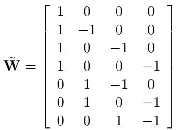
The comparison structure can be represented by a matrix \(\mathbf{W}\). For a comparison between item \(i\) and item \(j\), the row in the matrix has a \(+1\) at index \(i\) and a \(-1\) at index \(j\).

Using this matrix structure, the paper derives a beautiful closed-form solution for the optimal scores \(\hat{s}\):

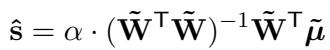
In this equation:

• \(\mathbf{W}\) is the comparison matrix (who played whom).
• \(\tilde{\boldsymbol{\mu}}\) is the vector of score differences predicted by the LLM probabilities.
• \(\alpha\) is a scaling factor.

This formula allows the system to instantly calculate the optimal ranking of all texts after every new comparison is made, which is crucial for efficiency.

Validating the Assumptions

The Gaussian expert assumes that the “true” score difference relates linearly to the LLM’s predicted probability. Is this actually true?

The researchers analyzed the data by comparing the LLM’s predicted probabilities against ground-truth human scores.

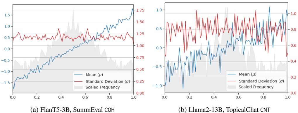
As shown in Figure 10 above:

1. Linearity (Blue line): The relationship between the LLM probability (x-axis) and the mean score difference (y-axis) is strikingly linear. As the model becomes more confident (probability moves toward 1.0), the actual score difference increases proportionally.
2. Constant Variance (Red line): The standard deviation (\(\sigma\)) remains relatively constant across the probability range.

These empirical findings validate the “Linear Gaussian” assumption, confirming that the fast, closed-form solution is not just mathematically convenient, but also grounded in reality.

Handling Bias

A known issue with pairwise comparisons is Positional Bias. LLMs often prefer the first option presented (e.g., “Answer A”) simply because it appears first.

The PoE framework handles this elegantly by introducing a bias term \(\beta\). If the model is unbiased, the expected probability for a random pair should be 0.5. If the model is biased (e.g., it averages 0.6 probability for the first position), we can shift the Gaussian mean to compensate.

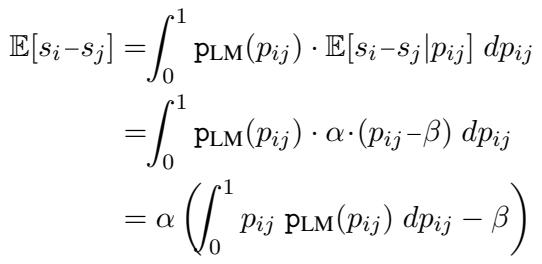
By setting \(\beta\) to the average probability output by the LLM over the dataset, the framework effectively “de-biases” the scores without needing to run every comparison twice (A vs B and B vs A), saving 50% of the compute.

Smart Comparison Selection

If we can’t afford to compare every single pair of texts, which pairs should we compare?

Because the Gaussian framework provides a closed-form expression for the uncertainty (covariance) of the scores, we can mathematically determine which next comparison would reduce the overall uncertainty the most.

The goal is to choose the pair \((i, j)\) that maximizes the determinant of the information matrix. The paper derives a greedy selection rule:

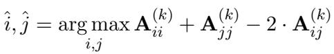
Here, \(\mathbf{A}\) is the inverse covariance matrix. This formula allows the system to actively select the most informative comparisons—usually pairs where the current estimated scores are uncertain or where the items are believed to be close in quality.

Experimental Results

The researchers evaluated their framework on several standard NLG datasets, including SummEval (summarization) and TopicalChat (dialogue). They compared the PoE method against standard baselines like Win-Ratio (simply counting wins) and standard Bradley-Terry.

Efficiency Gains

The most critical result is how quickly the method converges to the correct ranking.

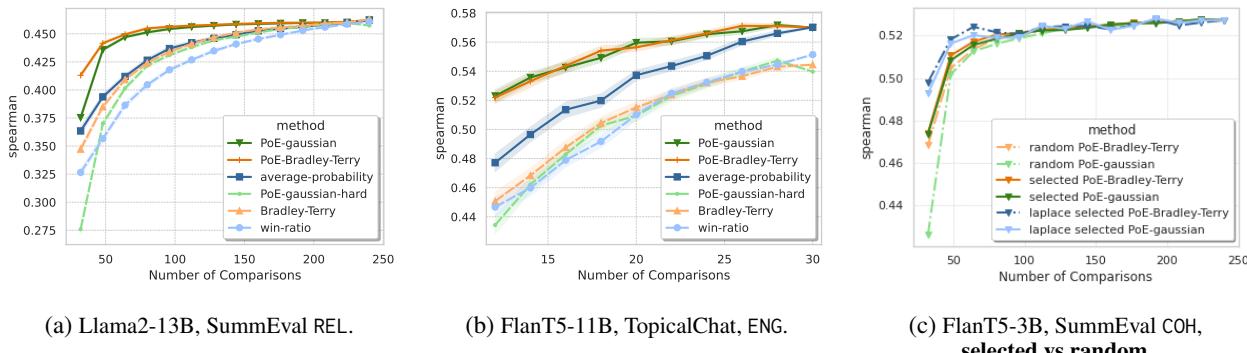
Figure 1 (above) tells the story:

• The Win-Ratio (light blue) is slow to improve. It needs many comparisons to get a decent correlation.
• The PoE approaches (Gaussian and BT, green and red lines) shoot up almost immediately. With only a small fraction of comparisons (low \(K\)), they achieve correlations nearly identical to using the full set of comparisons.

For example, on SummEval, using just 20% of the comparisons, the PoE method achieves a correlation score that the Win-Ratio method only achieves after using 100% of the comparisons.

Large Scale Performance

The method shines even brighter on large datasets. On the HANNA dataset (story generation) with over 1,000 candidates, the “all-pairs” comparison is impossible (over 1 million comparisons).

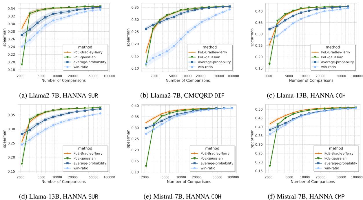
As shown in Figure 6, even with thousands of items, the PoE-Gaussian approach (green) and PoE-BT (orange) converge to high accuracy much faster than the baselines. They offer a practical way to rank large leaderboards without bankrupting the evaluator.

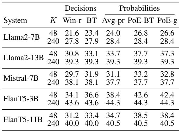
Summary of Performance

The table below summarizes the Spearman correlations on SummEval. Notice how the PoE methods (far right columns) consistently outperform Win-Ratio and Average Probability, especially when \(K\) (number of comparisons) is small (\(K=48\)).

Conclusion

The “LLM-as-a-judge” paradigm is here to stay, but the brute-force approach of comparing every pair is unsustainable. This paper introduces a sophisticated yet practical solution.

By viewing comparisons as a Product of Experts, we can:

1. Leverage Uncertainty: Use the soft probabilities from LLMs rather than just binary decisions.
2. Compute Fast: Use Gaussian experts to derive a closed-form solution that requires simple matrix math rather than iterative optimization.
3. Save Money: Achieve high-quality rankings using as few as 2% to 20% of the total possible comparisons.

This framework transforms pairwise evaluation from a computationally exhaustive task into a highly efficient, mathematically grounded process. For students and researchers looking to evaluate their own models, this implies that you don’t need a massive budget to get precise rankings—you just need the right math.

References: Liusie, A., Fathullah, Y., Raina, V., & Gales, M. J. F. “Efficient LLM Comparative Assessment: A Product of Experts Framework for Pairwise Comparisons.” University of Cambridge.