](https://deep-paper.org/en/paper/2405.12801/images/cover.png)
In the world of Information Retrieval (IR) and Natural Language Processing (NLP), we are constantly balancing two opposing forces: speed and accuracy.
When you type a query into a search engine or a chatbot, you expect an answer in milliseconds. To achieve this, systems rely on fast, lightweight models. However, you also expect that answer to be perfectly relevant. Achieving high relevance usually requires heavy, complex models that “read” every candidate document deeply.
For years, the industry standard has been a two-stage pipeline: Retrieve (fast but messy) and Rerank (slow but precise). But this pipeline has a flaw. If the fast retriever misses the right answer, the precise reranker never sees it. If we try to fix this by sending more candidates to the reranker, the system becomes too slow.
In this post, we will dive into a research paper that proposes a clever solution to this dilemma: Comparing Multiple Candidates (CMC). This framework introduces a way to compare a query against a batch of candidates simultaneously, allowing them to “see” each other and contextually fight for the top spot—all without sacrificing the speed of lightweight models.
The Problem: The Lonely Bi-Encoder and the Expensive Cross-Encoder
To understand CMC, we first need to understand the current architecture of modern search systems.
1. The Bi-Encoder (The Fast Retriever)
The first line of defense is usually a Bi-Encoder (BE). It processes the Query and the Candidate Document separately.
- It encodes the Query into a vector.
- It encodes the Candidate into a vector (usually pre-computed offline).
- It calculates a simple dot product (similarity score) between them.
The Pros: It is incredibly fast. You can search millions of documents in milliseconds using vector search indices. The Cons: It is “lonely.” The query representation doesn’t know about the candidate, and the candidate doesn’t know about the query until the very end. This lack of interaction often leads to lower accuracy.
2. The Cross-Encoder (The Accurate Reranker)
The top results from the Bi-Encoder are passed to a Cross-Encoder (CE).
- It feeds both the Query and the Candidate text into a BERT-like model together.
- The model’s self-attention mechanism allows every token in the query to interact with every token in the document.
The Pros: It is highly accurate because it deeply understands the relationship between the specific query and the document. The Cons: It is computationally expensive. Running a full BERT pass for every single candidate is slow. Therefore, we can only afford to rerank a small list (e.g., the top 10 or 50).
The Gap
This creates a bottleneck. If the Bi-Encoder puts the correct answer at position #60, and the Cross-Encoder only looks at the top 50, the system fails. We need a way to look at more candidates with high accuracy but without the massive computational cost of a Cross-Encoder.
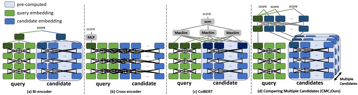
As shown in Figure 1 above:
- (a) Bi-Encoder: Fast, separate processing.
- (b) Cross-Encoder: Slow, deep interaction.
- (c) Late Interaction (like ColBERT): Better, but requires storing massive indices of token embeddings.
- (d) CMC (Ours): The proposed method. Note how the query interacts with multiple candidates (blue blocks) simultaneously in a shared space.
The Core Method: Comparing Neighbors Together
The researchers propose CMC (Comparing Multiple Candidates). The core insight is simple yet profound: We are better at making decisions when we can compare options side-by-side.
Standard models look at a (Query, Candidate) pair in isolation. CMC looks at a (Query, Candidate 1, Candidate 2, …, Candidate K) set. It uses a lightweight self-attention mechanism to let the candidates “interact” with the query and with each other.
1. Encoding the Input
First, CMC uses standard encoders to turn the query and the candidates into vector representations (embeddings). Crucially, the candidate embeddings are pre-computed. This maintains the efficiency of Bi-Encoders because we don’t need to re-encode the text of millions of documents at runtime.
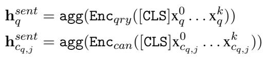
Here, Enc represents a transformer encoder (like BERT). We take the [CLS] token (a special token representing the whole sentence) to get a single vector for the query (\(h_q\)) and each candidate (\(h_c\)).
2. The Self-Attention Layer
This is where the magic happens. Instead of calculating a score immediately, CMC concatenates the query embedding with a list of \(K\) candidate embeddings. It feeds this sequence into a shallow Transformer block (just 2 layers).

In this equation:
- The input is a sequence of vectors:
[Query, Cand_1, Cand_2, ..., Cand_K]. - The Self-Attention mechanism allows the model to update the representation of the Query based on the Candidates, and update the representation of each Candidate based on the other Candidates.
This contextualization is powerful. If two candidates are semantically similar, the attention mechanism can highlight the subtle differences that make one a better fit for the query than the other.
3. Scoring
After the self-attention layers, we have “contextualized” embeddings. We then simply calculate the dot product between the updated query vector and the updated candidate vectors to find the best match.
The Full Architecture
Let’s visualize the entire process.
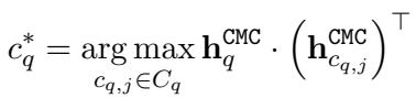
Figure 2 illustrates the flow:
- Retrieve: A standard Bi-Encoder retrieves a set of potential candidates.
- CMC: The pre-computed embeddings for these candidates are fetched.
- Process: The Query vector and these Candidate vectors act as the input to the CMC Transformer.
- Output: A refined, re-ordered list.
Because the candidate embeddings are just single vectors (not full lists of tokens like in ColBERT), the memory footprint is tiny. Because the transformer is shallow and processes inputs in batches, it is incredibly fast.
Training the Model
To teach CMC how to distinguish between good and bad candidates, the researchers use a loss function that combines standard classification accuracy with “distillation”—meaning it also tries to learn from the probability distribution of the original retriever.
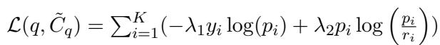
The first part of the equation (\(\lambda_1\)) is the standard Cross-Entropy loss (find the right answer). The second part (\(\lambda_2\)) uses KL-Divergence to ensure the model doesn’t drift too far from the original retriever’s logic, acting as a regularizer.
Hard Negative Sampling To make the model robust, you can’t just show it easy examples. The researchers use “Hard Negatives”—incorrect candidates that look very similar to the query according to the Bi-Encoder.
By forcing the model to distinguish the correct answer from these “tricky” incorrect ones, CMC learns fine-grained distinctions.
The “Seamless” Intermediate Reranker
One of the most compelling use cases for CMC is plugging it into the middle of the existing pipeline.
Currently, we have: Bi-Encoder \(\to\) Cross-Encoder. The proposal is: Bi-Encoder \(\to\) CMC \(\to\) Cross-Encoder.
Why add a step? Doesn’t that make it slower? Surprisingly, no.
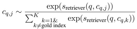
As shown in Figure 3:
- (a) Standard: The Bi-Encoder retrieves \(M\) candidates. The Cross-Encoder is so slow it can only process those \(M\). If the answer isn’t in \(M\), you lose.
- (b) With CMC: The Bi-Encoder retrieves a much larger set \(K\). CMC is fast enough to process all \(K\) candidates and filter them down to the best \(K'\) (where \(K' \approx M\)).
The Cross-Encoder still only has to process a small number of candidates, but those candidates are of much higher quality because they were pre-filtered by CMC. You catch the gold nuggets that the Bi-Encoder would have missed, without slowing down the final ranking.
Experimental Results
The researchers tested CMC on several challenging datasets, including ZeSHEL (Zero-Shot Entity Linking) and MS MARCO (Passage Ranking).
1. Better Retrieval Performance
When acting as a retriever (or intermediate reranker), does CMC actually find better documents?
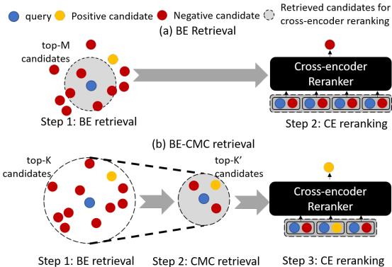
Table 1 shows the results on ZeSHEL.
- Look at Recall@64 (R@64). The standard Bi-Encoder achieves 88.0%.
- CMC pushes this to 91.5%.
- It outperforms other complex methods like Poly-encoder and Sum-of-max.
- Crucially, look at the Index Size. Sum-of-max requires 25.7 GB of storage. CMC requires only 0.4 GB—roughly the same as a standard Bi-Encoder.
2. Speed vs. Scalability
The claim is that CMC compares “neighbors together.” Does this scale?
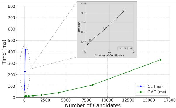
Figure 4 is perhaps the most important chart in the paper.
- The Blue Line (Cross-Encoder) shoots up vertically. Processing just a few hundred candidates takes hundreds of milliseconds.
- The Green Line (CMC) is nearly flat. It can process 10,000 candidates in roughly the same time it takes a Cross-Encoder to process 16.
This extreme efficiency is what makes the “intermediate reranking” strategy possible.
3. Versatility Across Tasks
CMC isn’t just for entity linking. It works for passage ranking and dialogue systems too.
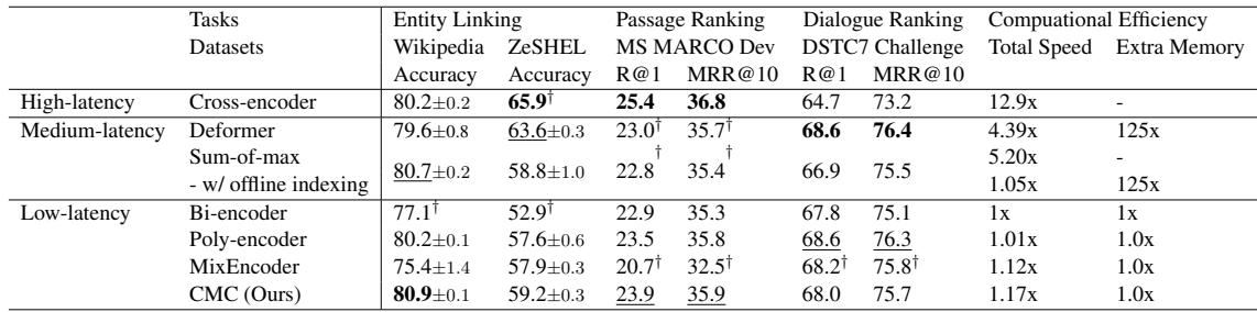
Table 3 compares CMC against high-latency (Cross-Encoder), medium-latency, and low-latency models.
- In Entity Linking, CMC actually outperforms the Cross-Encoder (80.9 vs 80.2), despite being 11x faster.
- In Dialogue Ranking (DSTC7), it also beats the Cross-Encoder significantly (68.0 vs 64.7).
- In Passage Ranking, it remains competitive with much heavier models while maintaining the speed profile of a Bi-Encoder.
4. Initialization Matters
An interesting finding in the ablation study was the effect of “Transfer Learning.”
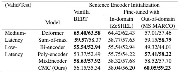
Table 4 shows that initializing the encoders with weights fine-tuned on a different domain (like MS MARCO) helps performance on ZeSHEL. This suggests that CMC benefits from robust, general-purpose sentence embeddings as a starting point.
Conclusion
The “Comparing Multiple Candidates” (CMC) framework offers a graceful solution to the classic trade-off in information retrieval. By shifting the perspective from “Does this document match this query?” to “Which of these documents best matches this query given the competition?”, CMC achieves a level of accuracy that rivals heavy Cross-Encoders.
However, its true strength lies in its efficiency. By utilizing pre-computed embeddings and shallow self-attention, it maintains the blazing speed of Bi-Encoders.
For students and practitioners building search systems, CMC offers two paths:
- The Accelerator: Replace your slow Cross-Encoder with CMC to make your system 10x faster with minimal accuracy loss.
- The Enhancer: Insert CMC before your Cross-Encoder to filter a massive pool of candidates, improving recall and catching difficult answers that simple vector search misses.
In a world where data volume is exploding, methods like CMC that compare neighbors jointly are likely to become the new standard for efficient, high-performance retrieval.