Learning to Learn, Cooperatively — How a Sparring Partner Boosts Meta-Learning

How can a machine learning model learn to recognize a new object from just one or two examples? Humans do this effortlessly. If you see a single picture of a “quetzal,” you can likely identify other quetzals later. For AI, this kind of challenge falls under few-shot learning—a notoriously difficult problem. The key lies in a fascinating concept called meta-learning, or “learning to learn.”

Instead of training one model on a massive dataset for a single task, meta-learning trains a model across many smaller tasks. The goal isn’t to master each task, but to master the process of learning itself. This way, when the model faces a new and unseen task with very little data, it can adapt quickly and perform effectively.

One of the most popular and influential meta-learning algorithms is Model-Agnostic Meta-Learning (MAML). MAML seeks an initialization of model weights that provides the perfect starting point for learning any new task. However, finding such truly general initialization parameters is challenging—the model often overfits to the training tasks, limiting its adaptability.

A recent paper, Cooperative Meta-Learning with Gradient Augmentation, presents a clever and effective improvement to MAML. It introduces a temporary co-learner during training that works alongside the main learner like a sparring partner—adding meaningful noise and diversity to the learning process. After training, this co-learner disappears, leaving behind a better, more generalizable model. The result? You get all the benefits without any additional inference cost.

In this article, we’ll unpack this cooperative framework, explore why it works so well, and discuss its implications for the future of learning systems.

---

Background: A Quick Primer on MAML

Before diving into the innovation of Cooperative Meta-Learning (CML), it helps to review MAML’s core mechanism.

MAML works through two nested optimization loops designed to teach a model how to learn from minimal data:

1. Inner Loop — Task Adaptation: For each specific learning task (for example, classifying cats vs. dogs), the model starts with the current meta-initialization parameters. Then, using a small support set of examples, it performs one or a few gradient descent updates. This produces new, task-specific parameters.

2. Outer Loop — Meta-Optimization: After adaptation, the model is evaluated on different examples—called the query set. The error on this set guides the update of the original meta-initialization parameters. This “meta-update” teaches the model how to learn efficiently, improving the starting point for future tasks.

Repeating this process across thousands of diverse tasks steers MAML’s parameters toward a globally effective initialization—one that quickly adapts to entirely new challenges.

In the typical setup, the model includes:

• a feature extractor \( \psi \), which handles data representation, and
• a meta-learner \( \theta \), which acts as the classifier or regressor built on top of those features.

---

The Core Method: Cooperative Meta-Learning (CML)

The authors noticed a limitation: the meta-gradients MAML computes during outer-loop optimization can be too narrow or overfit. What if these gradients were augmented in a structured way to encourage better generalization?

Enter the co-learner \( \phi \).

CML expands the network with this second classifier head, which shares the same feature extractor \( \psi \) as the meta-learner \( \theta \). The co-learner offers an alternate viewpoint, injecting learnable noise that regularizes the meta-optimization process.

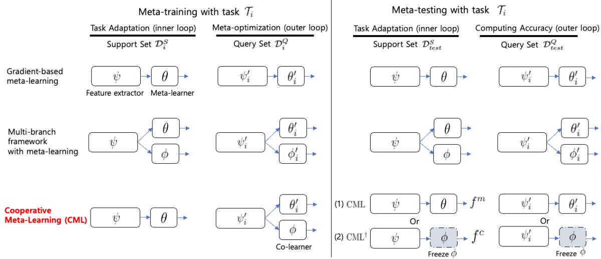
Figure 1: Overall schematic comparing gradient-based meta-learning, multi-branch frameworks, and the proposed Cooperative Meta-Learning (CML). During training, both the meta-learner \( \theta \) and co-learner \( \phi \) share the feature extractor \( \psi \). The co-learner participates only in the outer loop and is removed at test time.

---

The Asymmetric Training Process

CML’s magic lies in its asymmetric training procedure. Let’s follow one meta-training iteration.

1. Inner Loop: The Meta-Learner Adapts; The Co-Learner Waits

For a given task \( \mathcal{T}_i \) with support and query sets \( \mathcal{D}_i^S \) and \( \mathcal{D}_i^Q \):

Only the meta-learner \( \theta \) and feature extractor \( \psi \) are updated using the support set. The co-learner \( \phi \) remains frozen—it does not adapt to the task. This creates asymmetry.

\[ (\psi'_i, \theta'_i) \leftarrow (\psi, \theta) - \alpha \nabla_{(\psi, \theta)} \mathcal{L}(f^m_{(\psi, \theta)}; \mathcal{D}_i^S), \quad \phi'_i = \phi \]

Now, \( \theta \) holds task-specific knowledge while \( \phi \) retains meta-knowledge of previous tasks—two complementary perspectives.

2. Outer Loop: Cooperative Gradient Update

During the meta-update on the query set, both learners contribute to the total loss:

\[ \mathcal{L}_{total} = \sum_{i}^{N}\left[\mathcal{L}\left(f^m_{(\psi'_i, \theta'_i)}; \mathcal{D}_i^{Q}\right) + \gamma\, \mathcal{L}\left(f^c_{(\psi'_i, \phi)}; \mathcal{D}_i^{Q}\right)\right] \]

The gradient from both parts flows back through the shared feature extractor, combining the specialized and general viewpoints. This gradient augmentation produces a richer update that regularizes learning without external noise or pruning.

The overall meta-update becomes:

\[ (\psi, \theta, \phi) \leftarrow (\psi, \theta, \phi) - \beta \nabla_{(\psi, \theta, \phi)} \mathcal{L}_{total} \]

3. Meta-Testing: Streamlined Inference

Once training finishes, the co-learner \( \phi \) can be removed. The final model—consisting only of \( \psi \) and \( \theta \)—operates like the original MAML, meaning no extra computation or parameters at test time.

The authors also evaluated a variant called \( CML^{\dagger} \), which uses the co-learner for inference instead of the meta-learner. Remarkably, it performs equally well, proving that the shared feature extractor learns highly generalizable representations.

---

Experiments: Proving the Idea

The authors thoroughly test CML to answer three questions:

1. Does it outperform baseline methods?
2. Can it adapt to various data domains?
3. What explains its success?

---

Few-Shot Regression

First, they evaluate sinusoidal regression—predicting a sine wave given only a few sampled points.

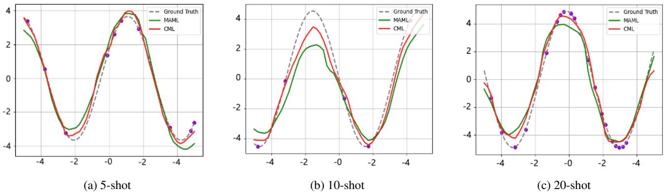
Figure 2: CML produces better fits than MAML in few-shot regression tasks, particularly in low-shot scenarios (leftmost panel).

Across 5-, 10-, and 20-shot tasks, the red CML curve aligns far more closely with the true sinusoid, showing that the cooperative learning process improves generalization even in simple settings.

---

Few-Shot Image Classification

CML was inserted into four popular MAML variants—original MAML, MAML++, BOIL, and Sharp-MAML—and evaluated on MiniImagenet.

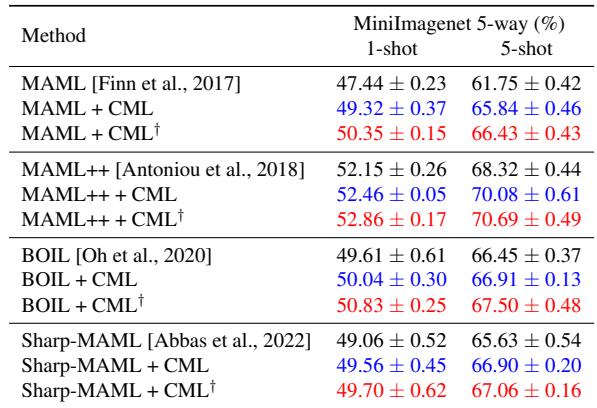
Table 1: Across all baselines, adding CML boosts accuracy. Notably, MAML++ + CML achieves 70.08% on the 5-shot task versus 68.32% for the original.

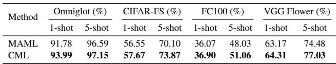
Table 2: Generalization holds across different datasets—CML improves results in every case without increasing inference cost.

These results show that CML can serve as a plug-in optimizer applicable to a wide family of gradient-based meta-learners.

---

Few-Shot Node Classification

To demonstrate versatility beyond images, the authors apply CML to graph-based learning tasks using G-Meta and AMM-GNN algorithms.

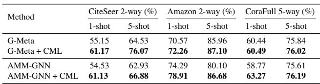
Table 3: CML enhances performance in graph-based few-shot node classification, proving compatibility with architectures like GNNs.

Again, CML consistently improves accuracy even on non-Euclidean graph domains, underscoring its generic regularization power.

---

Understanding Why CML Works

Quantitative improvements are great—but what truly drives them? The authors conducted a detailed analysis of CML’s gradients and representations.

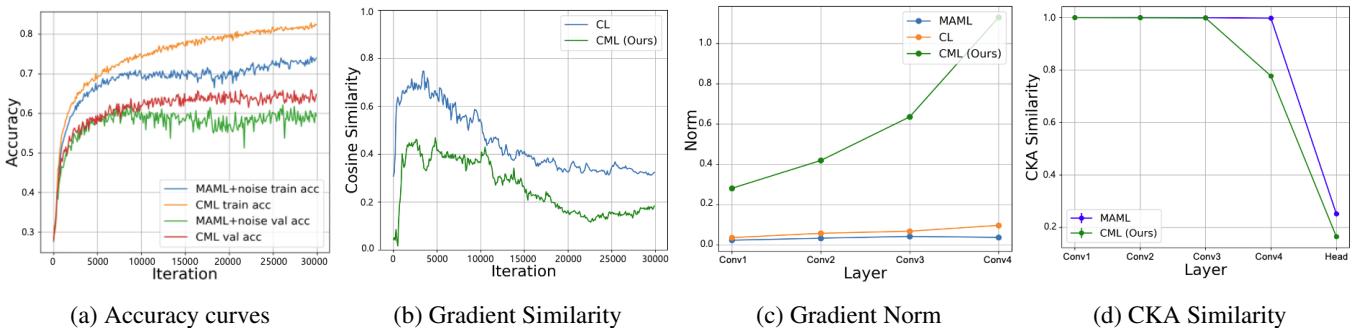
Figure 3: Analytical breakdown of CML’s learning dynamics. Each subpanel verifies how cooperative gradients enhance generalization.

(a) Structured Noise vs. Random Noise: Injecting random Gaussian noise into gradients improves generalization somewhat—but not as effectively as CML’s learned, meaningful noise from the co-learner.

(b) Gradient Diversity: CML maintains low gradient similarity between the meta-learner and co-learner, meaning the two are learning from distinct perspectives. This diversity stabilizes training and yields a richer gradient signal.

(c) Increased Gradient Norms: The larger gradient norms in the feature extractor indicate more substantial, dynamic changes—suggesting CML learns representations capable of adapting more flexibly.

(d) Representation Change via CKA: Using Centered Kernel Alignment (CKA) to compare representations before and after adaptation, CML shows deeper representation shifts than MAML. The feature extractor actually evolves with each task, not just the final classifier.

---

Is It Just About More Parameters?

To test whether CML’s success simply comes from having more parameters, the paper compares it to two larger baselines:

• More-MAML: A version of MAML with added layers.
• CL: A multi-branch training framework.

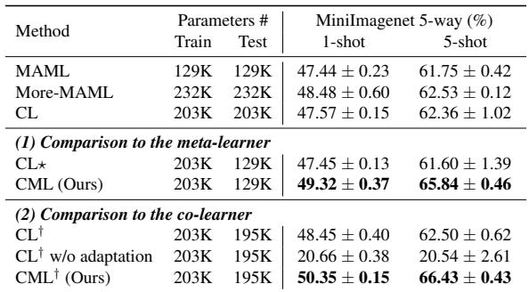
Table 4: Parameter comparison and test accuracy. CML beats both More-MAML and CL, confirming improvements aren’t due to model size.

The evidence is clear—CML’s structure, not parameter count, drives improvement.

---

Visualizing Learned Representations

Finally, t-SNE visualizations reveal how feature representations cluster after adaptation.

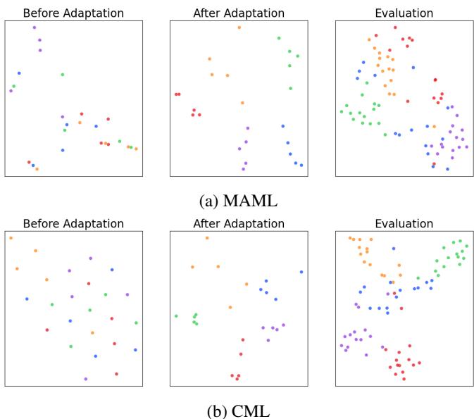
Figure 4: CML yields cleaner, more separated clusters, confirming its learned features generalize better across tasks.

These plots visually capture CML’s advantage: more coherent, separable feature spaces mean stronger classification boundaries and greater generalization.

---

Conclusion

The Cooperative Meta-Learning with Gradient Augmentation (CML) framework demonstrates that better generalization can come from cooperation, not complexity. By adding a non-adapting co-learner during training, it augments gradients with a meaningful form of learned noise, promoting diversity and robustness.

Key Takeaways:

1. A Novel Regularizer: CML’s gradient augmentation leverages cooperative interactions rather than random perturbations to improve meta-optimization.

2. Universal Applicability: The approach enhances a wide range of gradient-based meta-learning algorithms across domains—images, graphs, and regression alike.

3. Zero Inference Cost: The co-learner exists only during training; CML’s inference phase is as lightweight as MAML’s.

This paper illustrates a broader truth in machine learning: sometimes, improvement isn’t about adding more data or capacity—it’s about learning from diverse perspectives. Cooperative Meta-Learning embodies that philosophy, pointing toward future research where models may routinely train with collaborative partners to achieve sharper, more generalizable intelligence.