](https://deep-paper.org/en/paper/2406.05326/images/cover.png)
Introduction
In the world of Natural Language Processing (NLP), determining whether two sentences mean the same thing is a cornerstone task. Known as Semantic Textual Similarity (STS), this capability powers everything from search engines and recommendation systems to plagiarism detection and clustering.
For years, the industry has oscillated between two major paradigms. On one side, we have Sentence-BERT, a reliable architecture that encodes sentences independently. On the other, we have the modern heavyweights of Contrastive Learning (like SimCSE), which have pushed state-of-the-art performance to new heights.
However, a persistent problem remains. Contrastive learning models generally view the world in binary terms: sentences are either “similar” (positive) or “dissimilar” (negative). But human language is rarely that black and white. Sentences can be “somewhat related,” “mostly similar but differing in detail,” or “completely irrelevant.” By forcing these nuances into binary buckets, or by treating similarity scores as independent classification categories, we lose valuable information.
A recent paper by researchers from Tsinghua University, titled “Advancing Semantic Textual Similarity Modeling,” proposes a shift in perspective. Instead of treating similarity as a classification problem, they model it as a regression problem. To make this work, they introduce a novel neural architecture and two mathematically innovative loss functions: Translated ReLU and Smooth K2 Loss.
In this post, we will deconstruct their approach, explaining how treating similarity as a continuous spectrum—with a “buffer zone” for errors—can outperform traditional methods while using a fraction of the computational resources.
Background: The Current STS Landscape
To appreciate the innovation in this paper, we first need to understand the two dominant approaches currently used in the field.
1. The Siamese Network (Sentence-BERT)
The standard way to compare two sentences is to use a “Siamese” network structure (Bi-encoder). You feed Sentence A into a BERT model and Sentence B into the same BERT model (sharing parameters). You get a vector embedding for each. You then compare these vectors to determine similarity.
Sentence-BERT historically treated this as a classification task. If you had a dataset like NLI (Natural Language Inference) with labels like “Contradiction,” “Neutral,” and “Entailment,” the model would output a probability distribution across these three discrete classes.
2. Contrastive Learning (SimCSE)
More recently, Contrastive Learning has taken over. This method pulls the embeddings of similar sentences closer together in vector space while pushing dissimilar ones apart. While effective, it suffers from two main issues:
- Binary limits: It usually ignores fine-grained labels (e.g., a similarity score of 3 out of 5) and only focuses on the extremes (0 vs 5).
- Resource hunger: To work well, contrastive learning needs large batch sizes (often 512+) to see enough “negative” examples at once. This requires massive GPU memory.
The researchers argue that we can achieve the efficiency of Sentence-BERT with the performance of Contrastive Learning by fundamentally changing the objective of the training: Similarity should be regression, not classification.
The Core Method: A Regression Framework
The intuition here is simple: Semantic similarity is progressive. A score of 4 is closer to 5 than a score of 1 is. If a model predicts a “Neutral” relationship (score 1) when the truth is “Entailment” (score 2), that is a smaller error than predicting “Contradiction” (score 0).
Standard classification loss functions (like Cross-Entropy) treat all classes as independent; they don’t understand that Class 2 is “closer” to Class 3 than Class 5 is. Regression fixes this.
1. The Architecture
The authors propose a modified Siamese network. Let’s look at the architecture:
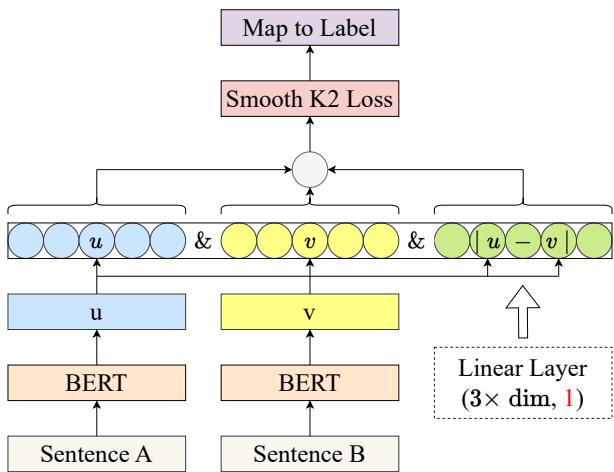
As shown in Figure 1, the process flows as follows:
- Input: Two sentences, A and B.
- Encoding: Both pass through a pre-trained BERT encoder to produce embeddings \(u\) and \(v\).
- Feature Engineering: The model concatenates three elements:
- The vector \(u\)
- The vector \(v\)
- The element-wise difference \(|u - v|\) (This captures the “distance” features between the sentences).
- The Regression Head: This concatenated vector is passed through a fully connected linear layer.
- Crucial change: Unlike classification models that output \(K\) nodes (one for each class), this model has only one output node.
This single node outputs a continuous floating-point number representing the similarity score.
2. The “Buffer Zone” Concept
If we are treating this as regression, why not just use standard Mean Squared Error (MSE) or L1 Loss?
Here is the subtle insight: The ground truth labels are often discrete points. In a 5-point similarity scale, the labels are 0, 1, 2, 3, 4, 5. If the true label is 3, and the model predicts 2.9, standard regression loss would penalize the model for that 0.1 difference.
However, if we round 2.9, we get 3. The classification is correct! Penalizing a model that is “close enough” is counter-productive. It forces the model to obsess over exact floating-point matches rather than learning general semantic patterns.
To solve this, the authors introduce a Zero-Gradient Buffer Zone. If the prediction is within a certain distance (threshold) of the true label, the loss is zero. The model is effectively told, “Good job, that’s close enough.”
3. Loss Function A: Translated ReLU
The first proposed solution is Translated ReLU. It modifies the standard L1 Loss (absolute difference) by shifting the activation function.
If the distance between the prediction and the label is less than a threshold \(x_0\), the loss is 0. If it exceeds that threshold, the loss increases linearly.
\[ \begin{array} { l } { x \mathrm { a b s } ( \mathrm { p r e d i c t i o n - l a b e l } ) \geq 0 } \\ { f ( x ) = \{ \begin{array} { l l } { 0 \quad x < x _ { 0 } \leq \frac { d } { 2 } } \\ { k ( x - x _ { 0 } ) \quad x _ { 0 } \leq x } \end{array} } \\ { f ( x ) = \operatorname* { m a x } \bigl ( 0 , k ( x - x _ { 0 } ) \bigr ) } \end{array} \]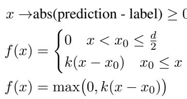
Here, \(d\) represents the interval between categories (e.g., if labels are 1, 2, 3, then \(d=1\)). As long as the error is less than half the interval (\(d/2\)), the rounded classification will be correct.
4. Loss Function B: Smooth K2 Loss
While Translated ReLU works, it has a sharp “corner” where the loss turns on. This abrupt change in gradient can sometimes make training unstable.
To smooth this out, the authors propose Smooth K2 Loss. This function also has a buffer zone of zero loss, but when the error exceeds the threshold \(x_0\), it rises quadratically (like a curve) rather than linearly.
\[ \begin{array} { c } { { f ( x ) = \{ \displaystyle { 0 \quad x < x _ { 0 } \leq \frac { d } { 2 } } \quad x _ { 0 } \leq x } } \\ { { k ( x ^ { 2 } - 2 x _ { 0 } x + x _ { 0 } ^ { 2 } ) \quad x _ { 0 } \leq x } } \\ { { \frac { \partial f ( x ) } { \partial x } = \{ \displaystyle { 0 \quad x < x _ { 0 } \leq \frac { d } { 2 } } \qquad } } \\ { { 2 k ( x - x _ { 0 } ) \quad x _ { 0 } \leq x } } \end{array} \]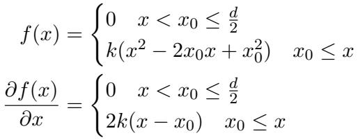
This quadratic rise means the model is penalized lightly for being slightly outside the buffer zone, but heavily for being far outside it. This dynamic gradient adjustment helps the model prioritize the worst predictions.
Visualizing the Difference
The graph below compares the two.
- Left: Translated ReLU. Flat, then a straight line up.
- Right: Smooth K2 Loss. Flat, then a curved line up.
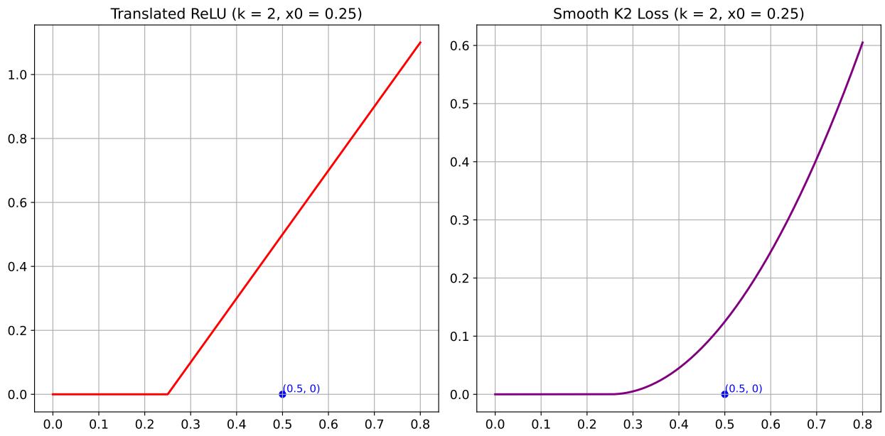
The authors found that Smooth K2 Loss generally performed better on high-quality datasets because of its ability to provide differentiable, adaptive gradients.
Experiments and Results
The researchers tested their framework on seven standard STS benchmarks (STS 12-16, STS-B, and SICK-R). They compared their regression approach against the traditional Sentence-BERT classification approach.
1. Regression vs. Classification
The results were compelling. In the table below (Table 1 from the paper), we can see the Spearman correlation scores (higher is better).
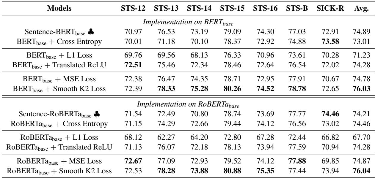
Key Takeaways from the Data:
- Regression Wins: Models trained with Translated ReLU or Smooth K2 Loss consistently outperformed the standard Cross-Entropy (classification) approach.
- Buffer Zones Matter: The new loss functions outperformed standard L1 Loss and MSE Loss. This proves that demanding exact floating-point matches hurts performance in STS tasks. The “buffer zone” allows the model to generalize better.
- Smooth K2 Supremacy: The Smooth K2 Loss achieved the highest average scores (76.03 on BERT-base), suggesting that the smoother gradient transition is indeed beneficial.
2. Boosting Contrastive Learning Models
One of the most exciting findings in the paper is that this regression framework isn’t just a replacement for old models—it can enhance the newest, most powerful ones.
Modern models like Jina Embeddings v2 and Nomic Embed use contrastive learning. The researchers took these pre-trained giants and fine-tuned them using their regression framework on specific, fine-grained STS data.
The process involves a two-stage fine-tuning setup:
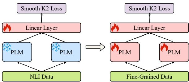
- Stage 1: Freeze the pre-trained language model (PLM). Only train the new linear output layer using general NLI data.
- Stage 2: Unfreeze the PLM and train the whole network using fine-grained STS data (with the Smooth K2 Loss).
The results of this hybrid approach are shown below:
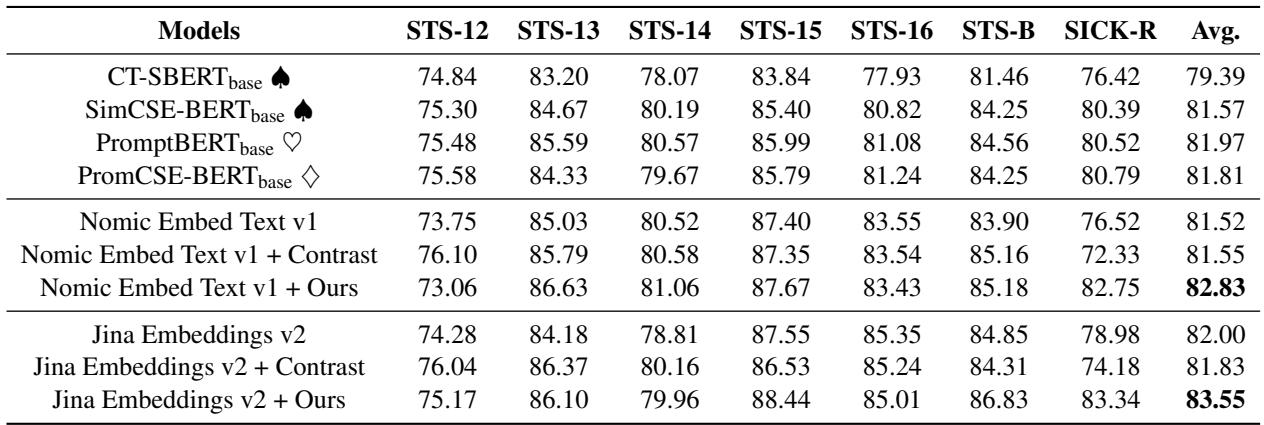
Notice the row “Jina Embeddings v2 + Ours” and “Nomic Embed Text v1 + Ours”. Both show clear improvements over the base models and even over models further fine-tuned with contrastive learning ("+ Contrast"). This highlights a major limitation of contrastive learning: because it relies on binary positive/negative pairs, it throws away the nuance of “moderately related” sentences. The regression framework captures that nuance.
3. Efficiency
Finally, let’s talk about computational cost. Contrastive learning (like SimCSE) requires massive batch sizes to prevent “model collapse” (where the model maps everything to the same point). SimCSE often uses a batch size of 512.
Because the regression framework processes pairs independently (or in small batches), it is incredibly efficient.
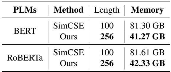
As shown in Table 4, SimCSE requires over 81 GB of memory to train with a sequence length of 100. The proposed regression method uses half that memory (41 GB) while supporting a sequence length of 256 (2.5x longer!). This makes high-performance STS modeling accessible to researchers with consumer-grade hardware.
Conclusion
The research paper “Advancing Semantic Textual Similarity Modeling” offers a refreshing step back from the complexity of massive contrastive learning setups. By identifying that semantic similarity is inherently a progressive, continuous concept, the authors successfully argue for a return to Siamese architectures powered by regression.
The key innovations—Translated ReLU and Smooth K2 Loss—provide the mathematical flexibility required to treat discrete labels as continuous targets. By incorporating a zero-gradient buffer zone, these loss functions prevent the model from overfitting to exact values, allowing it to focus on understanding semantic distance.
For students and practitioners, the takeaways are clear:
- Don’t ignore the nature of your labels. If your classes have an order (Good, Better, Best), classification loss might be suboptimal.
- Loss functions can be creative. Modifying standard losses to include margins or buffer zones can significantly impact performance.
- Efficiency matters. This regression framework achieves state-of-the-art results without requiring a cluster of industrial GPUs.
This work paves the way for smarter, leaner, and more nuanced text understanding models, bridging the gap between rigid classification and resource-heavy contrastive learning.