Introduction: Hitting the Wall in NLP

If you have been following the progress of Natural Language Processing (NLP), particularly in the realm of Sentence Embeddings, you might have noticed a trend. We have moved from simple word vectors like GloVe to sophisticated transformer-based models like BERT, and now to massive Large Language Models (LLMs) like LLaMA and Mistral.

Sentence embeddings are the backbone of modern AI applications. They convert text into numerical vectors, allowing computers to understand that “The cat sits on the mat” is semantically similar to “A feline is resting on the rug.” This technology powers everything from Google Search to Retrieval-Augmented Generation (RAG) systems.

The standard way to measure the quality of these embeddings is Semantic Textual Similarity (STS). We use benchmarks (like the SentEval toolkit) to see how well a model’s similarity scores correlate with human judgments.

For years, the scores kept going up. But recently, we hit a wall.

Take a look at the current state of the art:

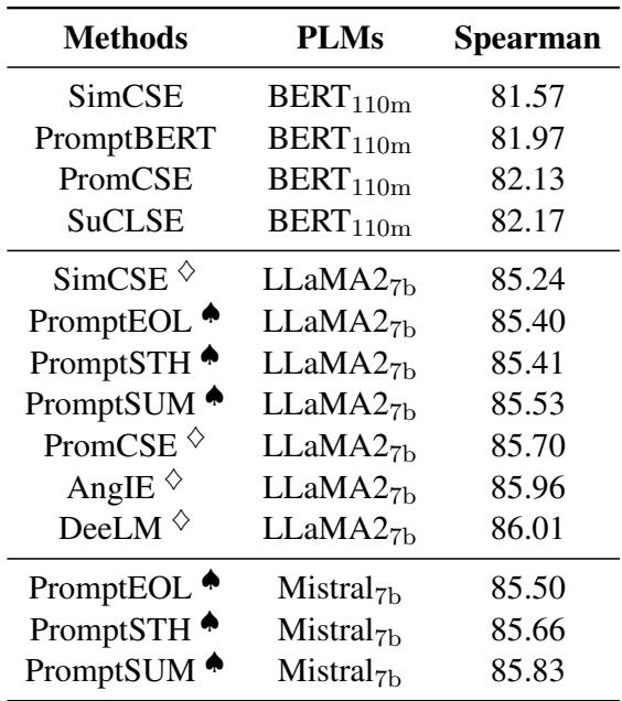
Whether researchers use BERT (110M parameters) or massive LLaMA models (7B parameters), and regardless of the prompt engineering or contrastive learning tricks they employ, the average Spearman’s correlation score seems stuck around 86.5.

Is 86.5 just the limit of what LLMs can understand? Or is there a fundamental flaw in how we are training them?

In this post, we are doing a deep dive into a fascinating paper titled “PCC-tuning: Breaking the Contrastive Learning Ceiling in Semantic Textual Similarity.” This research doesn’t just propose a new model; it mathematically proves that our current favorite training method—Contrastive Learning—has a theoretical performance ceiling of 87.5.

More importantly, the authors propose a solution, Pcc-tuning, which changes the rules of the game to break through this ceiling.

Background: The Era of Contrastive Learning

To understand why we hit a ceiling, we first need to understand the ladder we climbed to get here. The dominant paradigm in sentence representation today is Contrastive Learning.

The intuition behind contrastive learning is simple and elegant:

1. Take a sentence (Anchor).
2. Create a “positive” version of it (e.g., by using dropout noise or a paraphrase).
3. Treat other sentences in the batch as “negatives.”
4. Train the model to pull the Anchor and Positive close together in vector space while pushing the Negatives away.

The most popular loss function for this is InfoNCE Loss.

In this equation:

• The numerator calculates the similarity between the sample \(x_i\) and its positive pair \(x_i^+\).
• The denominator sums the similarity between \(x_i\) and all other samples (negatives).
• By minimizing this loss, we maximize the similarity of the positive pair relative to the negatives.

This approach, popularized by methods like SimCSE, revolutionized the field. It allowed models to learn robust semantic spaces without needing expensive, manually labeled data for every single sentence pair.

However, the authors of today’s paper argue that this strength is also its greatest weakness.

The Theoretical Ceiling: Why 87.5?

This is the most ground-breaking part of the research. The authors asked a critical question: How does Contrastive Learning actually view semantic similarity?

Contrastive Learning as a Binary Classifier

When we use InfoNCE loss, we are essentially telling the model to perform a binary classification task:

• Class 1 (Positive): This pair is similar.
• Class 0 (Negative): This pair is dissimilar.

The model is trained to distinguish between “Self” (positive) and “Others” (negative). It is not explicitly trained to say “Sentence A is 80% similar to Sentence B, but only 40% similar to Sentence C.” It creates a coarse-grained distinction.

Ideally, a perfect contrastive learning model acts like an Optimal Binary Classifier.

As shown in the figure above, a perfect binary classifier splits the data into two distinct chunks. It assigns a high similarity score (let’s say 1) to the top \(k\) most similar pairs and a low score (let’s say 0) to the remaining \(n-k\) pairs.

The problem? Human semantic similarity is not binary. It is a continuous spectrum. By forcing the model to learn a binary distinction, we limit its ability to rank sentences precisely.

Deriving the Limit

To prove this limitation, the authors look at the metric used to evaluate these models: Spearman’s Correlation Coefficient (\(\rho\)).

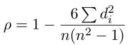
Spearman’s correlation measures rank order. It doesn’t care about the raw values, only that if humans rank Pair A higher than Pair B, the model should too. The variable \(d_i\) represents the difference between the human rank and the model’s rank for the \(i\)-th item.

If our Contrastive Learning model acts as an optimal binary classifier, it effectively groups the data into two blocks. Within the “positive” block, the model thinks all pairs are equally similar (ranking tied). Within the “negative” block, it thinks all pairs are equally dissimilar.

The authors mathematically modeled the rank differences (\(d_i\)) for this binary scenario:

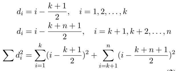
Here, the model classifies the first \(k\) items as positives and the rest as negatives. Even in this “perfect” binary scenario, the model makes ranking errors because it cannot distinguish within the positive group or within the negative group.

By expanding the summation of the squared differences (\(\sum d_i^2\)), they derive a function dependent on \(n\) (total samples) and \(k\) (the threshold for positive samples):

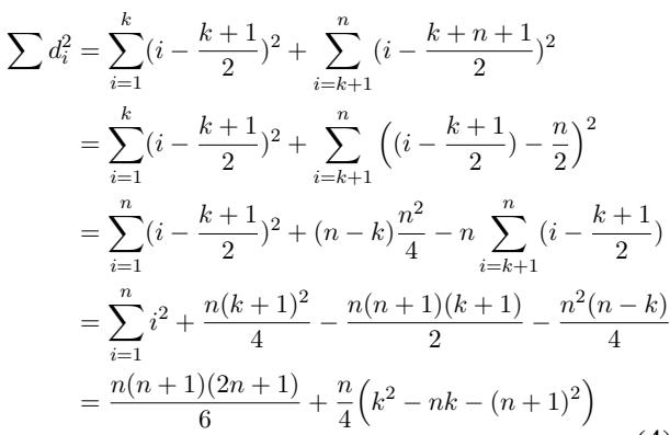
To find the best possible performance, we need to minimize this error. It turns out the error is minimized when \(k = n/2\)—that is, when the binary classifier treats exactly half the dataset as positive and half as negative.

Plugging this optimal state back into the Spearman formula:

Finally, taking the limit as the dataset size \(n\) goes to infinity, we arrive at the theoretical upper bound:

The result is 0.875.

This derivation is profound. It suggests that as long as we rely solely on standard Contrastive Learning (which behaves like a binary classifier), we are mathematically prevented from achieving a Spearman correlation higher than 87.5. The plateau at ~86.5 observed in Table 1 isn’t a failure of the models; it’s a fundamental property of the loss function.

The Solution: Pcc-tuning

To break a ceiling imposed by the loss function, we must change the loss function. The authors propose Pcc-tuning (Pearson Correlation Coefficient tuning).

The idea is to stop treating similarity as a binary classification problem (Similar vs. Not Similar) and start treating it as a regression problem that respects the continuous nature of semantic relationships.

The Two-Stage Architecture

Pcc-tuning employs a two-stage training pipeline.

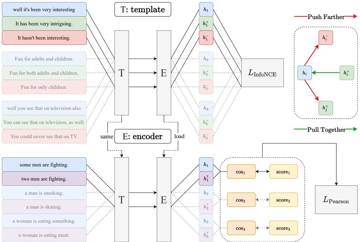
Stage 1: Contrastive Pre-training (The Warm-up)

We cannot simply ditch contrastive learning. It is incredibly effective at creating a uniform semantic space and fixing the “anisotropy” problem (where embeddings collapse into a narrow cone) common in PLMs.

• Method: The model is fine-tuned on a large Natural Language Inference (NLI) dataset using standard InfoNCE loss.
• Result: This gives us a strong “base” model that understands general semantic relationships but is still limited by the binary ceiling.

Stage 2: Pcc-tuning (The Refinement)

This is where the magic happens.

• Data: A small amount of fine-grained annotated data (specifically, filtered training sets from STS-B and SICK-R). We are talking about ~5,000 text pairs, which is tiny compared to the hundreds of thousands used in Stage 1.
• Loss Function: Instead of InfoNCE, the model minimizes the negative Pearson Correlation Coefficient.

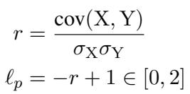
In this equation:

• \(X\) represents the cosine similarities predicted by the model.
• \(Y\) represents the continuous human-annotated scores (e.g., 4.2/5.0).
• \(r\) is the Pearson correlation between them.
• The loss is \(\ell_p = -r + 1\). Minimizing this maximizes the correlation.

By directly optimizing for correlation, the model learns the fine-grained nuances that contrastive learning ignores. It learns that a pair with a score of 4.5 should be closer than a pair with a score of 3.0, rather than just grouping them both as “positive.”

Experiments and Results

Does the theory hold up in practice? The authors tested Pcc-tuning across several 7B-parameter models (OPT, LLaMA, LLaMA2, Mistral).

Breaking the Ceiling

The results show that Pcc-tuning consistently pushes performance beyond the previous State-of-the-Art (SOTA).

While previous methods like PromptEOL and DeeLM hovered around 85-86, Pcc-tuning achieves scores like 87.86 on Mistral-7b. This effectively breaks the theoretical ceiling of 87.5 derived for contrastive methods.

Quality vs. Quantity: Pcc-tuning vs. Contrastive Learning

A skeptic might ask: “Maybe the improvement is just because you added more data in Stage 2?”

To test this, the authors compared Pcc-tuning against a “Two-Stage Contrastive” approach. In the comparison setup, they took the same Stage 1 model and continued training it on the Stage 2 data, but kept using Contrastive Loss (treating high-score pairs as positive).

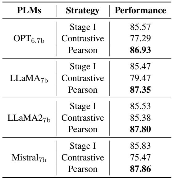
The results in Table 3 are stark:

• Contrastive: Continuing with contrastive learning actually hurt performance (scores dropped to ~85.5 or lower). This is likely because contrastive learning requires large batches and massive data to work well.
• Pearson (Pcc-tuning): Using the Pearson loss skyrocketed the performance to 87+.

This proves that the method (changing the loss function), not just the data, is the key to the improvement.

Robustness: Prompts and Batches

One of the frustrations with LLM-based embeddings is “Prompt Engineering”—spending hours finding the perfect phrase to trigger the model.

Pcc-tuning appears to be highly robust to different prompts. The authors tested three templates (PromptEOL, PromptSUM, PromptSTH).

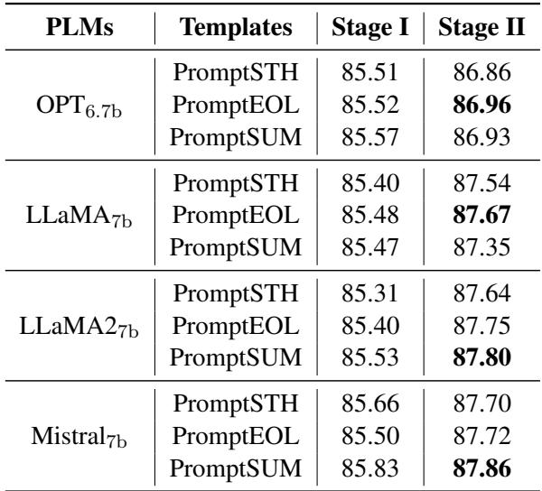
As shown in Table 5, regardless of whether the prompt asks for a “summary,” “one word,” or “something,” the Stage 2 fine-tuning (rightmost column) consistently yields scores around 87.3 - 87.8.

Furthermore, Pcc-tuning is efficient. Contrastive learning usually demands massive batch sizes (e.g., 512+) to find enough “hard negatives.” Pcc-tuning works on the correlation of the current batch.

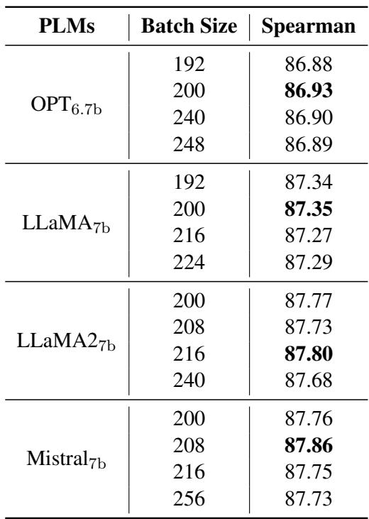
Table 8 shows that Pcc-tuning remains stable and effective even as batch sizes vary significantly. It also requires less memory because the correlation calculation is computationally lighter than the massive matrix operations required for large-batch contrastive learning.

Conclusion: A New Paradigm for Embeddings?

The paper “PCC-tuning: Breaking the Contrastive Learning Ceiling in Semantic Textual Similarity” offers a compelling narrative for the NLP community.

1. Diagnosis: It identifies that Contrastive Learning, while powerful, inherently limits STS performance to a score of 87.5 because it simplifies a continuous problem into a binary one.
2. Cure: It introduces Pcc-tuning, a method that aligns the training objective (Pearson Loss) with the evaluation objective (Correlation).
3. Efficiency: It achieves record-breaking results using a tiny fraction of data (less than 2% of the original training set size) for the second stage.

For students and practitioners, the takeaway is clear: Loss functions matter. When your model hits a plateau, it might not be a lack of data or model size—it might be that your training objective fundamentally disagrees with your end goal. By moving from binary discrimination to continuous correlation, Pcc-tuning unlocks the full granular potential of Large Language Models.

If you are working on sentence embeddings, it might be time to stop just “pushing and pulling” vectors and start looking at the correlation.