Introduction

We have all experienced the frustration of voice assistants failing us. In a quiet living room, they understand us perfectly. But try dictating a message while walking past a construction site or sitting in a noisy café, and the system crumbles.

This phenomenon is known as domain shift. Deep learning models for Automatic Speech Recognition (ASR) are typically trained on relatively clean, controlled data. When deployed in the real world, they encounter “out-of-domain” samples—noisy environments they weren’t prepared for.

To fix this, researchers have turned to Test-Time Adaptation (TTA). The idea is simple but powerful: instead of freezing the model after training, let it continue to learn and adapt to the incoming audio during inference.

However, current TTA methods face a dilemma. Some reset themselves after every sentence (forgetting valuable context), while others try to learn continuously but risk “collapsing” or getting confused when the environment changes abruptly.

In this post, we will dive into a recent research paper that proposes a “best of both worlds” solution: a Fast-slow TTA framework called DSUTA. We will explore how it mimics the way humans learn—quickly adapting to immediate stimuli while slowly building long-term knowledge—and how a clever “Dynamic Reset” strategy keeps the model from going off the rails.

Background: The Dilemma of Adaptation

Before understanding the new solution, we need to understand the two prevailing approaches to Test-Time Adaptation.

1. Non-Continual TTA

Imagine a student taking a test where, for every single question, they are allowed to briefly look at the textbook, answer the question, and then undergo a memory wipe before the next question.

This is Non-continual TTA. The model adapts its parameters for the current audio clip (utterance), makes a prediction, and then resets to its original pre-trained state.

• Pro: It is very stable. If the model makes a mistake on one clip, it doesn’t affect the next one.
• Con: It is inefficient. It cannot leverage knowledge learned from previous clips, even if they were recorded in the exact same noisy environment.

2. Continual TTA (CTTA)

Now imagine the student keeps their memory throughout the test. As they answer questions about a specific topic, they get better at it.

This is Continual TTA. The model updates itself continuously stream-by-stream.

• Pro: It leverages cross-sample knowledge, improving performance over time in a consistent environment.
• Con: It suffers from error accumulation and model collapse. If the model starts making bad predictions, it trains itself on those errors, spiraling into failure. Furthermore, if the environment suddenly changes (e.g., leaving a quiet room and entering a noisy bus), the model might be “overfit” to the quiet room and fail to adapt to the bus.

Figure 1: A visual comparison of TTA approaches. On the left, Non-Continual TTA resets (\(\phi_0\)) every step. In the middle, Continual TTA passes the updated state forward indefinitely. On the right, the proposed Fast-slow approach blends both.

The Core Method: Fast-Slow TTA

The researchers propose a framework that bridges the gap between these two extremes. They call it Fast-slow TTA.

The intuition is derived from the fact that we need two types of updates:

1. Fast Adaptation: We need to adjust parameters quickly to handle the specific noise in the current sentence.
2. Slow Evolution: We need to slowly update a set of “meta-parameters” that capture the general characteristics of the current environment (e.g., the hum of an air conditioner) without overfitting to a single sentence.

The Mathematical Framework

The Fast-slow framework is elegant in its separation of concerns. It introduces meta-parameters (\(\phi_t\)) that serve as the starting point for adaptation.

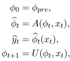
Here is what is happening in the equations above:

1. Initialization: We start with pre-trained parameters (\(\phi_{pre}\)).
2. Fast Adaptation (\(A\)): When a new data sample \(x_t\) arrives, we create a temporary version of the model, \(\widehat{\phi}_t\). This version is “fast” because it is aggressively adapted to fit just this current sample.
3. Prediction: We use this temporary, fast-adapted model to make the prediction \(\widehat{y}_t\).
4. Slow Update (\(U\)): Simultaneously, we use the new data to perform a “slow” update on the meta-parameters \(\phi_t\) to get \(\phi_{t+1}\). These meta-parameters become the starting point for the next sample.

By doing this, the model has a “better start” for every new sample because the meta-parameters (\(\phi\)) have learned from the past, but the specific prediction is made by a version (\(\widehat{\phi}\)) that is tightly optimized for the current moment.

Dynamic SUTA (DSUTA)

The researchers implemented this framework using a method called Dynamic SUTA (DSUTA). It uses an unsupervised objective function called Entropy Minimization—essentially trying to make the model more confident in its predictions (sharpening the output probability distribution).

In DSUTA:

• The Adaptation (\(A\)): Performs \(N\) steps of optimization on the current sample to minimize entropy.
• The Update (\(U\)): Uses a small buffer (memory) of the last \(M\) samples. Every \(M\) steps, it updates the meta-parameters using the average loss from this buffer. This mini-batch approach stabilizes the “slow” learning process.

Handling The Real World: Dynamic Reset Strategy

While Fast-slow TTA solves the issue of learning from past data, it introduces a new risk. What if the user walks from a quiet library onto a loud street? The “slow” meta-parameters are tuned for the library. When the street noise hits, the model might fail to adapt because its starting point is too far off.

Standard Continual TTA fails here. The solution proposed in this paper is the Dynamic Reset Strategy.

Figure 2: The complete architecture. Notice the “Domain Shift Detection” block. If a shift is detected, the meta-parameters are reset to the original source model (Clean Slate). If not, they continue to update slowly.

Detecting the Shift

How does the model know the environment has changed without being told? It needs a metric—an unsupervised indicator that screams “This data looks weird!”

The researchers devised the Loss Improvement Index (LII).

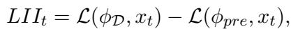
The logic behind LII is clever:

1. \(\mathcal{L}(\phi_{\mathcal{D}}, x_t)\): Calculate the loss of the current sample using the model adapted to the current domain.
2. \(\mathcal{L}(\phi_{pre}, x_t)\): Calculate the loss of the current sample using the original pre-trained model.
3. Subtract them.

Why subtract? Because some sentences are just naturally harder to recognize than others, regardless of background noise. Subtracting the pre-trained loss acts as a normalization step, canceling out the inherent difficulty of the speech content. This leaves us with a value that purely reflects how well the current domain adaptation fits the incoming audio.

To make the detection robust, they don’t look at just one sample (which is noisy). They average the LII over the buffer size (\(M\)).

Figure 3: This histogram proves the effectiveness of LII. The Blue distribution (In-domain) is distinct from the Orange distribution (Out-of-domain). This separation allows us to set a statistical threshold.

The Reset Mechanism

The system alternates between two stages:

1. Domain Construction: When a reset happens, the system spends some time (\(K\) steps) building a statistical profile (mean and variance) of the LII for this new environment. It basically learns “what normal looks like” for this specific noise.
2. Shift Detection: Once the profile is built, it checks every incoming batch. If the LII deviates significantly (using a Z-score test) from the profile, it triggers a reset.

Figure 4: The timeline of adaptation. The model adapts (green icons), builds a domain profile, monitors for shifts, and when the ‘Out domain’ sample hits (red), it resets to the pre-trained weights (\(\phi_{pre}\)) and starts over.

The mathematical logic for the reset is defined as:

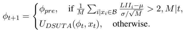
If the Z-score of the current buffer’s LII is greater than 2 (meaning it is statistically very unlikely to belong to the current domain), the meta-parameters \(\phi_{t+1}\) are hard-reset to \(\phi_{pre}\). Otherwise, the standard DSUTA update continues.

Experiments and Results

The researchers tested this approach rigorously using Librispeech mixed with various noises (like vacuum cleaners, cafes, and street noise) and the CHiME-3 dataset (real-world noisy recordings).

1. Single Domain Performance

First, they tested a scenario where the noise is consistent (Single Domain).

Table 1: Word Error Rate (WER) comparison. Lower is better.

The results in Table 1 are striking:

• Source Model: 40.6% error on “AA” (Airport Announcement) noise.
• SUTA (Non-continual): Improves to 30.6%.
• DSUTA (Proposed): Drastically reduces error to 25.9%.

DSUTA outperforms the baselines in almost every category. This confirms that carrying over knowledge (the “slow” update) provides a massive benefit over resetting every time.

Why is it better? The researchers analyzed the adaptation process and found that DSUTA essentially gives the optimization a head start.

Figure 5: The “Better Start” effect. The orange line (DSUTA) consistently stays lower (better) than the blue line (SUTA) and the baseline, indicating that the meta-parameters are successfully accumulating useful knowledge.

2. Time-Varying Domains

This is the most critical test. The researchers created “Multi-domain” datasets where the noise type changes sequentially (e.g., from AC noise to Typing noise to Airport noise).

• MD-Easy: Sequences of noises where the model usually performs well.
• MD-Hard: Sequences of difficult noises.
• MD-Long: A long sequence (10,000 samples) with random lengths, simulating a long day of usage.

Table 2: Performance on shifting domains.

Key Takeaways from Table 2:

1. Standard Continual TTA fails: Look at “CSUTA” on MD-Long. It hits 100.3% WER. This is model collapse in action. The model got confused and never recovered.
2. DSUTA is robust: Even without the dynamic reset, DSUTA performs well (43.2% on MD-Long).
3. Dynamic Reset is King: Adding the dynamic reset (“w/ Dynamic reset”) drops the error further to 35.8%.

Interestingly, the Dynamic Reset strategy sometimes outperformed the “Oracle boundary” (where the model is told exactly when the noise changes). This suggests that sometimes, retaining knowledge across slightly different domains is better than a hard reset, and the Dynamic strategy is smart enough to decide when to keep knowledge and when to dump it.

3. Efficiency

One might assume that all this buffer calculation and statistical tracking makes the model slow. Surprisingly, it’s the opposite.

Table 3: Efficiency comparison.

Because DSUTA starts with better meta-parameters, it requires fewer adaptation steps (\(N\)) to reach a good result compared to SUTA. As shown in Table 4, DSUTA is significantly faster in total runtime (3885s vs 5040s for SUTA) while achieving higher accuracy.

Conclusion

The transition of ASR models from the lab to the real world is fraught with challenges, primarily due to unpredictable background noise. This paper presents a compelling step forward with Dynamic SUTA.

By adopting a Fast-slow TTA framework, the authors successfully combined the stability of single-sample adaptation with the cumulative learning benefits of continual adaptation. The addition of the Dynamic Reset Strategy solves the “catastrophic forgetting” vs. “model collapse” trade-off, allowing the system to detect environmental shifts autonomously.

The implications are significant for edge AI. We are moving toward voice assistants that don’t just passively process audio, but actively learn and adjust to your environment in real-time, whether you are in a library or on a construction site.

Key Takeaways:

• Don’t Reset blindly: Keeping a memory of past samples (meta-parameters) improves accuracy.
• Don’t Remember blindly: Indefinite learning leads to collapse; you must know when to reset.
• Unsupervised indicators work: Using relative loss improvement (LII) is a viable way to detect domain shifts without labels.