Introduction

In the rapidly evolving landscape of Artificial Intelligence, Large Language Models (LLMs) have established themselves as the undisputed kings of knowledge and reasoning. From writing code to summarizing history, their capabilities are vast. However, a significant gap remains between generating text and taking optimal actions in a dynamic environment.

Consider a recommendation system, a healthcare triage bot, or a digital assistant. These are sequential decision-making problems. The agent observes a context, selects an action, and receives feedback (a reward or loss). Traditionally, we solve these with algorithms like Contextual Bandits. These algorithms are computationally cheap and learn well over the long term, but they suffer from the “cold start” problem—they begin with zero knowledge and must flail around randomly to learn what works.

On the other hand, LLMs start with massive amounts of “common sense” knowledge. They can make decent decisions immediately. But there is a catch: they are computationally expensive, slow, and static. They don’t naturally “learn” from user feedback without complex and costly finetuning.

So, we face a dilemma: do we choose the fast learner that starts stupid (Contextual Bandits), or the smart genius that is too expensive to run and doesn’t adapt (LLMs)?

In this post, we break down a fascinating paper titled “Efficient Sequential Decision Making with Large Language Models” by researchers from the University of South Carolina and UC Riverside. They propose a hybrid framework that acts as a bridge, utilizing the initial wisdom of LLMs to “warm up” a standard decision-making algorithm, before seamlessly handing over control to the cheaper, faster model. The result? A system that is statistically superior to both and computationally efficient.

Background: The Players

Before diving into the solution, let’s briefly define the two main components the researchers are trying to reconcile.

1. Sequential Decision Making (Contextual Bandits)

In a contextual bandit problem, an agent acts in rounds. In every round \(t\):

1. The agent sees a context \(x_t\) (e.g., a user’s profile and search history).
2. The agent chooses an action \(a_t\) (e.g., recommends a specific product).
3. The agent receives a loss or reward (e.g., did the user click?).

The goal is to minimize the total loss over time. The challenge is the exploration-exploitation tradeoff. The agent must explore new actions to find better ones but exploit known good actions to maximize reward. Standard algorithms (like SpannerGreedy) are great at this eventually, but they start with no knowledge, leading to poor initial performance.

2. LLMs as Agents

LLMs can be prompted to make decisions. For example, you can feed an LLM a product description and ask it to predict the correct category tag.

• Pros: They have immense prior knowledge. They don’t need to “learn” that a smartphone belongs in “Electronics”—they already know.
• Cons: They are massive. Running GPT-4 or even Llama 3 for every single user interaction in a high-traffic system is often cost-prohibitive and slow. Furthermore, updating them based on that single click (feedback) requires gradient updates (finetuning), which is incredibly expensive.

The Core Method: Online Model Selection

The researchers propose a framework that doesn’t force us to choose one or the other. Instead, they use Online Model Selection. Think of this as a “Manager” algorithm that sits above the LLM and the Contextual Bandit (CB).

In the beginning, the Manager knows the CB is untrained, so it delegates most decisions to the LLM. The LLM makes good choices, and crucially, the data generated by the LLM (context, action, and reward) is used to train the CB.

As the CB learns from this high-quality data, it starts improving. The Manager observes this improvement and gradually shifts the workload from the expensive LLM to the cheap, now-competent CB.

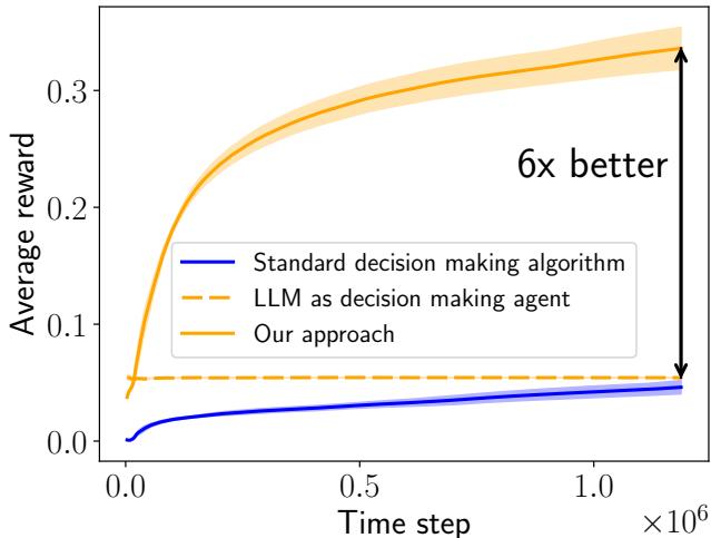
As shown in Figure 1 above, this approach (the orange solid line) combines the strengths of both. It avoids the low start of the standard algorithm (blue line) and surpasses the flat performance of the standalone LLM (dashed orange line), eventually achieving a 6x performance gain.

Step 1: Converting LLMs into Policies

One practical hurdle is that LLMs output text, while decision algorithms usually select from a discrete set of actions (like ID #452 or ID #901).

To fix this, the authors use an embedding-based approach (Algorithm 1 in the paper):

1. Prompt the LLM with the context (e.g., “Predict the item tag…”).
2. The LLM generates a text response.
3. This response is converted into a vector embedding.
4. The system calculates the similarity between this response vector and the embedding vectors of all possible valid actions.
5. The action with the highest similarity is chosen.

This allows any off-the-shelf LLM to function as a decision-making policy without any training.

Step 2: The Balancing Act

The heart of the paper is Algorithm 2. This is the loop that decides who gets to act.

At each time step \(t\):

1. The framework holds a probability distribution \(p_t\). This represents the probability of choosing the LLM vs. the Contextual Bandit.
2. It samples a choice based on \(p_t\).
3. The chosen agent acts, and a reward is observed.
4. Crucially: Regardless of who acted, the Contextual Bandit updates its internal model using the data. This means the Bandit learns even when the LLM is doing the work.
5. The framework updates \(p_t\) for the next round.

Step 3: Sampling Strategies

How do we update \(p_t\)? We want to rely on the LLM early on and fade it out later. The authors explore several strategies.

Simple Decay: The simplest method is to force the probability of using the LLM (\(p_t^{LLM}\)) to drop over time, either polynomially or exponentially.

Polynomial decay looks like this:

Exponential decay drops even faster:

Learning-Based (Log-Barrier OMD): While simple decay works, the authors prefer a more intelligent approach called Log-Barrier Online Mirror Descent (OMD). Instead of blindly reducing the LLM’s usage, OMD looks at the performance (losses) of both agents. It dynamically adjusts the probabilities based on which agent is actually performing better. If the Bandit is learning slower than expected, the system keeps the LLM involved longer.

Budget Constraints: Real-world systems often have a hard budget for LLM calls (e.g., “We can only afford 10,000 API calls”). The authors introduce a modification to strictly limit LLM usage:

Here, \(N_t\) is the number of calls made so far, and \(B\) is the budget. As the budget runs out, the probability of calling the LLM is forced to zero.

Experiments and Results

To validate this framework, the researchers tested it on two distinct datasets involving text-based decision making.

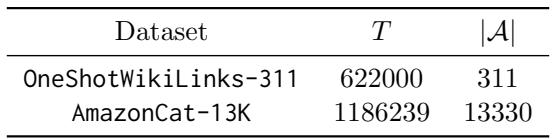
Table 1 outlines the datasets:

• OneShotWikiLinks-311: A Named-Entity Recognition task (311 possible actions).
• AmazonCat-13K: A massive multi-label classification task with over 13,000 possible actions (tags).

Statistical Efficiency: Higher Rewards

The primary metric is average reward (higher is better).

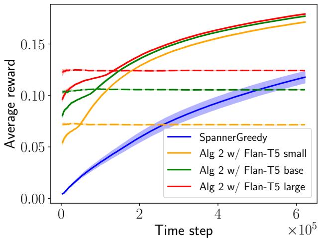
In Figure 2, we see the results on the WikiLinks dataset using Flan-T5 models of different sizes (Small, Base, Large).

• Blue Line (SpannerGreedy): The standard bandit algorithm starts poor and learns slowly.
• Dashed Lines: These are the pure LLMs. Note that the larger the model, the better the static performance, but they never improve.
• Solid/Dotted Lines (Algorithm 2): The proposed method shoots up immediately. Remarkably, Algorithm 2 with Flan-T5 Small (Orange Line) eventually outperforms the pure Flan-T5 Large (Red Dashed). This proves that a smart learning algorithm assisted by a weak LLM can beat a strong LLM acting alone.

Computational Efficiency: The Cost Factor

This is where the paper makes its strongest case for industry application. Running LLMs is expensive.

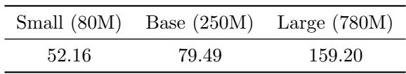
Table 2 shows the execution time disparity. A single decision by a Flan-T5 Large model takes nearly 160 times longer than the Contextual Bandit.

However, because the proposed framework shifts probability away from the LLM as the bandit learns, it rarely calls the LLM in the long run.

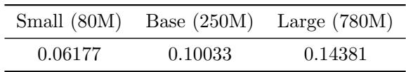
Table 3 reveals that over the course of the experiment, the LLM was called only 6% to 14% of the time. This is a massive resource saving compared to the 100% required by the “LLM as Agent” baseline.

Furthermore, when explicitly limiting the budget using the equation discussed earlier, the algorithm still holds up:

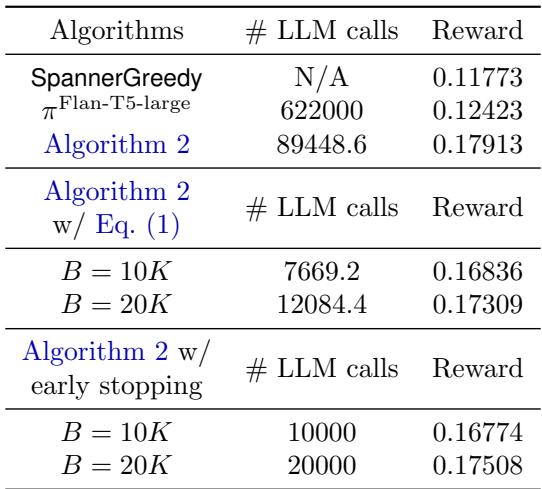
As seen in Table 4, even when capping the LLM calls to a strict budget (e.g., 10k calls out of 600k rounds), the reward remains significantly higher (0.168) than the standard bandit (0.117).

Does it work with modern LLMs?

The researchers didn’t just stop at T5. They tested the framework with Gemma 2B and GPT-4o-mini on the difficult AmazonCat dataset.

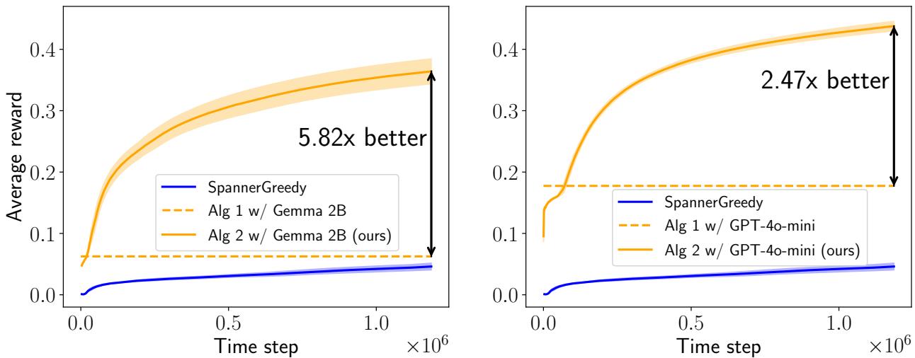
Figure 3 confirms the trend holds.

• Left (Gemma 2B): The hybrid approach (Solid Orange) dominates the baseline, achieving a 5.82x gain.
• Right (GPT-4o-mini): The hybrid approach achieves a 2.47x gain.

In both cases, the system benefits from the “reasoning” of the advanced models to guide the bandit through the complex action space of 13,000 items.

Why Does It Work? The Analysis

Why exactly does the hybrid model outperform both of its parents?

The hypothesis is that the LLM acts as a “teacher.” In a standard bandit setting, the algorithm explores randomly. In a large action space (like 13,000 tags), random exploration is useless—you will almost never hit the correct tag by chance.

However, the LLM, even if not perfect, narrows down the search space significantly. It suggests actions that are plausible. The bandit observes these “smart” interactions and updates its weights.

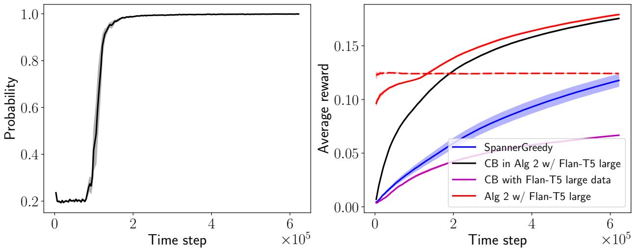
Figure 4 illustrates this dynamic beautifully:

• Left Graph: Shows the probability of using the Contextual Bandit (\(p_t^{CB}\)). It starts low but rapidly approaches 1.0. The system essentially “weans” itself off the LLM.
• Right Graph: The black line shows the hypothetical performance of the Bandit component if it were running alone but trained inside the hybrid loop. It learns incredibly fast. The Purple line shows a bandit trained only on LLM data. The gap between the Black and Purple lines suggests that the hand-off is vital. The Bandit eventually needs to take over and perform its own fine-grained exploration to surpass the teacher.

Conclusion and Implications

This research papers presents a compelling “Plug-and-Play” framework. It allows engineers to take an off-the-shelf LLM and a standard bandit algorithm and combine them to create a decision-making agent that is:

1. Smarter than traditional algorithms (avoids cold start).
2. More adaptable than pure LLMs (learns from feedback).
3. Cheaper than pure LLMs (reduces inference calls by >85%).

For students and practitioners, the takeaway is clear: We don’t always need to fine-tune massive models to get good results. Sometimes, the most efficient solution is to let the large model teach a smaller, specialized algorithm, getting the best of both worlds.

Comparison of Strategies

To wrap up, the authors compared how different probability update strategies impacted the final results.

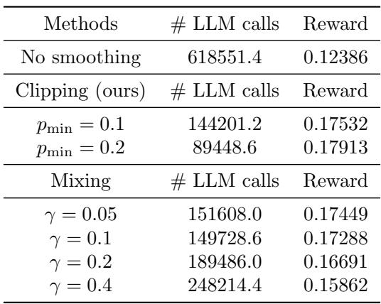
Table 5 and Table 6 highlight that while simple decay strategies work, the Log-barrier OMD (the adaptive strategy) yields the highest reward, and using a “clipping” smoothing strategy helps prevent the bandit from being ignored too early in the process.

This work paves the way for efficient AI agents that can operate in real-time environments without breaking the bank on inference costs.