Beyond Nodes and Edges: How GraphBridge Unifies Text and Structure in Graph Learning

In the evolving landscape of Machine Learning, we often find ourselves categorizing data into distinct types. We have Natural Language Processing (NLP) for text and Graph Neural Networks (GNNs) for networked structures. But the real world is rarely so tidy. In reality, data is often a messy, beautiful combination of both.

Consider a social network. You have users (nodes) and friendships (edges). But you also have the content those users generate—their bios, posts, and self-introductions. To truly understand a user, you can’t just look at who they know (structure), nor can you only look at what they write in isolation (text). You need to understand how their text relates to the text of the people they hang out with.

This specific data type is known as a Text-Attributed Graph (TAG). While we have methods to handle text and methods to handle graphs, bridging the gap between the detailed semantics of text and the broad context of graph structure has been a persistent challenge.

In this post, we are doing a deep dive into a fascinating paper titled “Bridging Local Details and Global Context in Text-Attributed Graphs.” The researchers introduce GraphBridge, a framework designed to seamlessly integrate these two worlds. Perhaps most impressively, they solve the massive computational headache that usually comes with mixing graphs and heavy text data: scalability.

The Problem: The Disconnected View

To understand why GraphBridge is necessary, we first need to look at how we currently handle Text-Attributed Graphs.

In a standard TAG, every node comes with a rich set of text. If you are classifying research papers in a citation graph, the node is the paper, and the text is the abstract.

Traditionally, researchers have treated this as a two-step assembly line:

1. Local-Level Encoding: We take the text of a node and pass it through a Language Model (like BERT) to turn it into a vector (a list of numbers). This captures the semantic meaning of the text.
2. Global-Level Aggregating: We take those vectors and feed them into a Graph Neural Network (like GCN). The GNN mixes the vector of a node with its neighbors. This captures the structural relationships.

While this works, it misses something crucial: Interconnection.

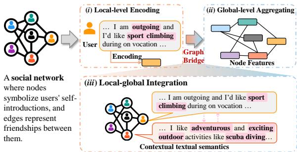
As shown in Figure 1 above, existing methods (steps i and ii) treat the text encoding and the graph structure as separate phases. Step iii illustrates what is missing: the contextual textual information.

Imagine you are at a party. If you introduce yourself as “I love climbing,” that’s your local text. If you are standing in a group of people, that’s your global structure. Current methods essentially record your “I love climbing” statement, and then note that you are standing near Bob and Alice.

But what if Bob’s profile says “I am an outgoing instructor” and Alice’s says “I organize outdoor adventures”? The semantic relationship between your “climbing” and their “outdoor adventures” is the key to understanding that you are likely part of a specific hobbyist group. GraphBridge aims to capture this specific nuance—the text-to-text relationship between connected nodes.

The Challenge: The Scalability Bottleneck

The intuitive solution to this problem seems simple: Why not just take the text from a node, append the text from all its neighbors, and feed that giant paragraph into a powerful Language Model (LLM)?

The answer is computational cost.

Language Models have a limit on how much text they can process (context length). If a node has 50 neighbors, and each neighbor has a 200-word bio, you are suddenly asking the model to process 10,000+ tokens for a single prediction. This leads to:

1. Memory Explosion: You will run out of GPU memory immediately.
2. Noise: Not every word in a neighbor’s text is relevant.
3. Dilution: The target node’s own information might get drowned out by the neighbors.

This is where GraphBridge introduces its core innovation: a mechanism to intelligently shrink the text while keeping the graph context.

The Solution: GraphBridge

The GraphBridge framework operates on a “Multi-Granularity Integration” philosophy. It connects the local (text) and global (graph) perspectives by ensuring that the Language Model actually “sees” the text of the neighbors.

To make this computationally feasible, the authors designed a Graph-Aware Token Reduction module.

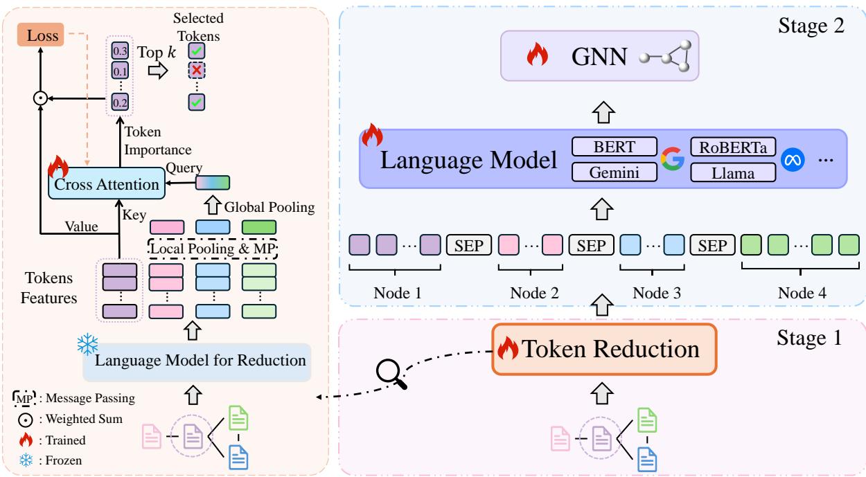
As illustrated in Figure 2, the process is split into two distinct stages. Let’s break them down.

Stage 1: Graph-Aware Token Reduction

The goal here is simple but difficult: Keep the words that matter, discard the ones that don’t. But “what matters” depends on the graph structure. A word in a neighbor’s text is only important if it helps classify the current node.

The authors devised a learnable attention mechanism to score every token (word/sub-word) based on both its semantic meaning and the graph structure.

Step A: Getting the Representations

First, they use a pre-trained Language Model (frozen, so it’s fast) to get embeddings for every token in a node. They average these to get a summary vector for the node, denoted as \(z_i\).

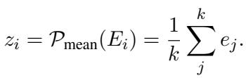
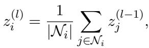
Next, they perform a Message Passing step (similar to how GCNs work). They average the summary vectors of a node’s neighbors. This creates a “Query” vector that represents the neighborhood context.

Step B: The Cross-Attention Score

This is the clever part. To decide which tokens in node \(i\) are important, the model asks: How well does this specific token align with the neighborhood context?

They calculate an importance score using a cross-attention mechanism:

• Query (\(Q\)): The aggregated neighborhood features (What is the context?)
• Key (\(K\)): The individual token embeddings (What is the content?)

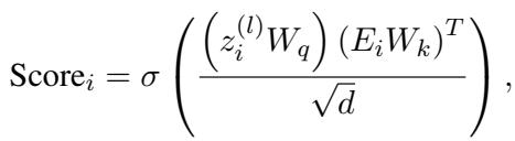
This formula outputs a probability score for every token. If a token has a high score, it means it is highly relevant to the surrounding graph structure.

Step C: Optimization and Regularization

The model selects the top-\(k\) tokens based on these scores. But how do we train this selector? We force it to solve the downstream classification task using only the weighted sum of these tokens.

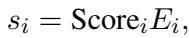
However, the researchers found a problem during testing. Without checks and balances, the model would “overfit” to specific words, assigning a score of 0.99 to one token and ignoring the rest. This creates a “tunnel vision” effect where the model relies on a single keyword rather than understanding the sentence.

To fix this, they added a Regularization term using KL-divergence. This forces the importance scores to be somewhat distributed, preventing the model from betting everything on one token.

The impact of this regularization is stark. Look at the chart below:

In Figure 3, the purple line (With Regularization) shows that the highest scores are distributed reasonably. The blue line (Without Regularization) shows that for almost all nodes, the model pushed the confidence of a single token to 1.0 (the far right), ignoring everything else.

The final training loss combines the task accuracy and this regularization:

Stage 2: Multi-Granularity Integration

Once the Token Reduction module is trained, we can compress the text data significantly. A long abstract might be reduced to just its 10-20 most critical keywords.

Now, we can finally do what we wanted to do at the start: Concatenate.

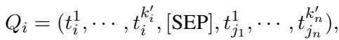
For a target node \(i\), GraphBridge constructs a new sequence \(Q_i\). This sequence contains:

1. The reduced tokens of the node itself.
2. A separator token [SEP].
3. The reduced tokens of its neighbors (sampled via a random walk).

Because the tokens are reduced, this sequence fits comfortably within the context window of a standard Language Model (like RoBERTa or even LLaMA).

The Language Model is then fine-tuned on this graph-enriched sequence:

Finally, the embeddings generated by this LM are passed into a standard GNN for the final classification. This cascading structure allows the GNN to benefit from the rich, context-aware text processing that happened upstream.

Experimental Analysis

Does this complex bridging actually work? The authors tested GraphBridge against a suite of baselines on seven standard datasets.

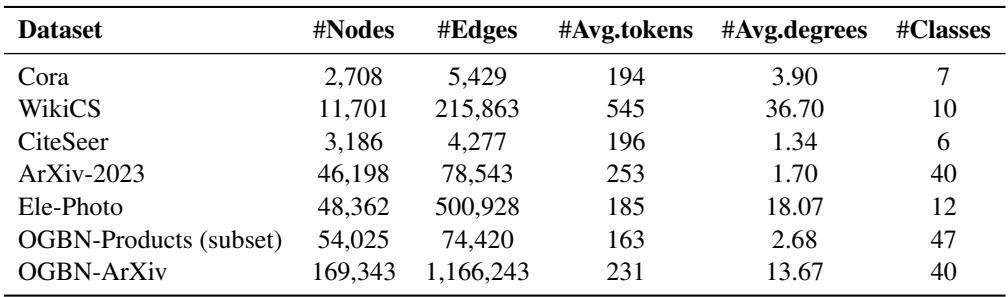
The Datasets

The datasets range from citation networks (Cora, ArXiv) to product graphs (OGBN-Products).

Performance Comparison

The results, shown in Table 2, are quite revealing.

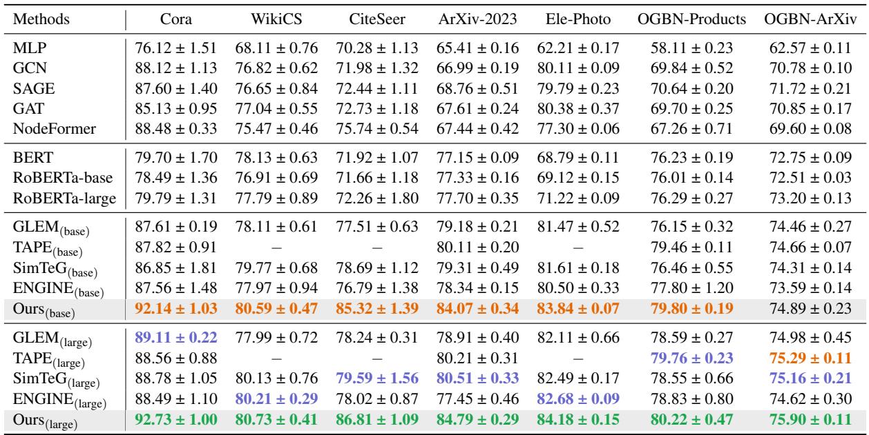
Here is what the data tells us:

1. GNNs vs. LMs: Traditional GNNs (GCN, SAGE) often struggle compared to methods that use Language Models (GLEM, SimTeG) because they ignore the rich text semantics.
2. The GraphBridge Advantage: GraphBridge (Ours) consistently outperforms the previous state-of-the-art methods. For example, on CiteSeer, GraphBridge (base) achieves 85.32% accuracy, jumping significantly ahead of SimTeG’s 78.69%. This suggests that “reading” the neighbor’s text allows the model to categorize nodes much more accurately than just aggregating vectors.

LLM Integration

The framework is model-agnostic. The authors swapped out RoBERTa for LLaMA2-7B, a much larger Generative LLM.

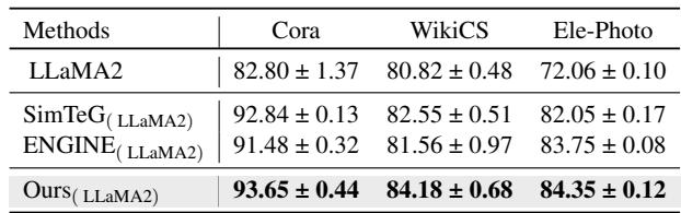
As seen in Table 3, GraphBridge with LLaMA2 achieves the highest scores across the board. This proves the method scales well with the capabilities of the underlying Language Model.

Scalability: The Real Winner

Perhaps the most practical contribution of this paper is efficiency. Training LMs on graph neighborhoods usually leads to Out-Of-Memory (OOM) errors.

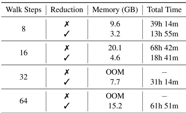
Table 4 shows the stark difference.

• Without Reduction: With 32 walk steps (neighbors), the model goes OOM. Even at 16 steps, it takes 68 hours and 20GB of memory.
• With Reduction: The model handles 32 steps easily, taking only 31 hours and 7.7GB of memory.

This reduction allows the model to “see” further into the graph (more neighbors) without crashing the hardware.

Ablation Studies

How do we know the “Smart” token reduction is better than just random selection or TF-IDF?

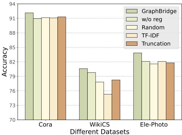
Figure 6 compares GraphBridge’s reduction (far left bars) against Random, TF-IDF, and simple Truncation. GraphBridge consistently wins. It also shows that the “w/o reg” (Without Regularization) version performs worse, confirming that the KL-divergence loss is necessary for stable learning.

Conclusion

GraphBridge represents a significant step forward in Graph Representation Learning. By acknowledging that text in a graph doesn’t exist in a vacuum, it effectively bridges the semantic gap between a node and its neighbors.

Its two-pronged approach—first intelligently reducing the noise via Graph-Aware Token Reduction, and then synthesizing that information via Multi-Granularity Integration—offers a blueprint for how to handle the increasingly complex data we see in the real world.

For students and practitioners, the key takeaways are:

1. Context is King: In TAGs, the text of a neighbor is as important as the link itself.
2. Less is More: You don’t need every word. If you can intelligently select the tokens that align with the graph structure, you can improve performance while slashing computational costs.
3. Regularization Matters: When designing attention mechanisms, always ensure your model isn’t collapsing its focus onto a single feature.

As we move toward Graph Foundation Models, techniques like GraphBridge that efficiently handle massive textual attributes will likely become the standard for processing the web’s interconnected data.