](https://deep-paper.org/en/paper/2406.13718/images/cover.png)
The current generation of Large Language Models (LLMs) often feels like magic. Ask a model like BLOOM or GPT-4 to translate French to English, and the result is usually flawless. Switch to Hindi, and it still performs admirably. But what happens when you step just slightly outside the spotlight of these “High-Resource Languages” (HRLs)?
There are approximately 7,000 languages spoken today, but LLMs are typically trained on a tiny fraction of them—usually around 100. The vast majority of the world’s languages, including thousands of dialects and closely related variations, are left in the dark.
Intuitively, we know that if an LLM knows Hindi, it should understand a bit of Maithili (a related language spoken in India and Nepal). If it knows German, it might grasp some Swiss German. This is the promise of cross-lingual generalization. But in practice, performance often falls off a cliff. Why? Is it because the spelling is different? Is it the grammar? Or is it simply that the vocabulary doesn’t overlap?
In this post, we are doing a deep dive into a fascinating paper by Bafna, Murray, and Yarowsky from Johns Hopkins University. They propose a novel framework to answer these questions by treating linguistic differences not as binary “different languages,” but as noise applied to a known language.
By synthetically generating thousands of “artificial languages,” they systematically pinpoint exactly what breaks an LLM.
The Problem: The HRL-CRL Gap
To understand the challenge, we first need to look at the relationship between a High-Resource Language (HRL) and its Closely-Related Languages (CRLs).
An HRL is a language with massive amounts of training data available (e.g., English, Spanish, Hindi). A CRL is a linguistic neighbor—it shares ancestry, vocabulary, and grammar, but has distinct variations.
LLMs suffer from Performance Degradation (PD) when moving from an HRL to a CRL. But measuring this is tricky because real low-resource languages often lack the evaluation datasets (like Q&A pairs or entailment datasets) needed to test the model. Furthermore, we rarely know if a “low-resource” language was actually lurking in the model’s training data, which muddies the results.
The researchers illustrate the complexity of these differences in Figure 1, comparing Hindi (HRL) and Maithili (CRL).
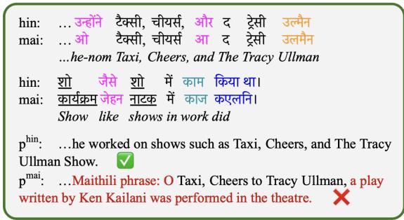
As shown above, the differences aren’t random. They fall into specific linguistic categories:
- Phonological: Sound changes that lead to spelling differences (e.g., teksi vs teksī).
- Morphological: Changes in word endings or grammar (e.g., unhoni vs o).
- Lexical: Different words entirely (e.g., kāma vs karyakṃ).
The core insight of this paper is brilliant in its simplicity: If we lack data for real dialects to test these dimensions, why not build them?
The Core Method: Synthesizing Languages via “Noising”
The researchers model the distance between languages as a Bayesian noise process. They take a source language (the HRL) and apply “noisers” to it. These noisers corrupt the text in linguistically plausible ways to create an artificial CRL.
By controlling the “volume” of this noise (represented by the parameter \(\theta\)), they can generate a spectrum of languages ranging from “almost identical” to “distant cousin.”
1. The Phonological Noiser (\(\phi^p\))
Languages evolve through sound shifts. For example, the ‘p’ sound in Latin (pater) shifted to ‘f’ in Germanic languages (father). This noiser mimics that process.
It doesn’t just swap letters randomly. The researchers use the International Phonetic Alphabet (IPA) to ensure changes are physically possible. They group sounds by their features (lip-rounding, voicing, aspiration).
As seen in the IPA character sets above, a sound like ‘p’ might change to ‘b’ (voicing change) or ‘f’ (manner change), but it likely wouldn’t spontaneously turn into a vowel like ‘a’.
The noiser works by converting the text to IPA, applying a change with probability \(\theta_p\) based on the surrounding context (left and right characters), and then mapping it back to the script. This simulates the regularity of sound change—if ’d’ changes to ’t’ at the end of a word, it tends to happen consistently across the language.
2. The Morphological Noiser (\(\phi^m\))
Morphology deals with the structure of words—specifically suffixes and prefixes. In related languages, the root of the word often stays the same (a “cognate”), but the grammatical ending changes.
The morphological noiser (\(\phi^m\)) identifies common suffixes in the source language. With probability \(\theta_m\), it replaces a suffix with a generated alternative. To keep things realistic, the new suffix is generated by taking the old suffix and applying heavy phonological noise to it. This creates a new ending that looks and sounds like it belongs in the same language family but is distinctly different.
3. The Lexical Noiser (\(\phi^{f,c}\))
Finally, sometimes words just change completely. This is lexical variation. The authors split this into two categories:
- Function Words (\(\phi^f\)): These are the glue of sentences—prepositions, pronouns, determiners (e.g., “the”, “in”, “he”). They are a closed set and highly frequent.
- Content Words (\(\phi^c\)): Nouns, verbs, adjectives. These carry the bulk of the meaning.
The noiser replaces these words with probability \(\theta_f\) or \(\theta_c\). The replacement isn’t a synonym; it’s a “non-cognate”—a word that looks nothing like the original. The replacement is generated to be phonologically plausible for the script (a “nonsense” word that looks real).
Measuring the Damage: Performance Degradation (PD)
Once an artificial language is generated, the researchers test the LLM on it. They define a metric called Performance Degradation (PD) to quantify how much the model suffers.
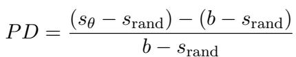
In this equation:
- \(s_{\theta}\) is the score on the noised (artificial) language.
- \(b\) is the baseline score on the original clean language.
- \(s_{\text{rand}}\) is the score you’d get by guessing randomly.
Essentially, \(PD\) represents the percentage of capability lost. If \(PD\) is 0%, the model handles the dialect perfectly. If \(PD\) is 100%, the model has degraded to random guessing.
Connecting to Reality: Posterior Computation
You might be asking: “Artificial languages are cool, but do they reflect reality?”
To bridge the gap, the authors developed a way to calculate the noise parameters (\(\theta\)) for real language pairs. By aligning words between a real HRL (e.g., Hindi) and a real CRL (e.g., Awadhi), they can estimate how much phonological, morphological, and lexical distance actually exists between them.
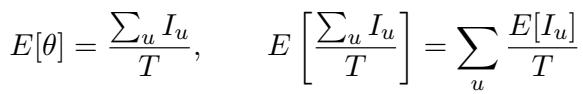
This equation allows them to calculate the expected noise \(\theta\) based on how many units (words, suffixes, or phonemes) differ between the source and the target language.
Experiments & Results
The team tested these noisers on the BLOOMZ-7b1 model using three tasks:
- Machine Translation (X \(\rightarrow\) eng): Translating the CRL into English.
- XNLI: Natural Language Inference (determining if a sentence implies another).
- XStoryCloze: Completing a story.
They experimented with 7 language families, including Hindi, Arabic, Indonesian, and German.
Result 1: Different Noises Hurt in Different Ways
The most compelling result is the visualization of how performance drops as noise increases.
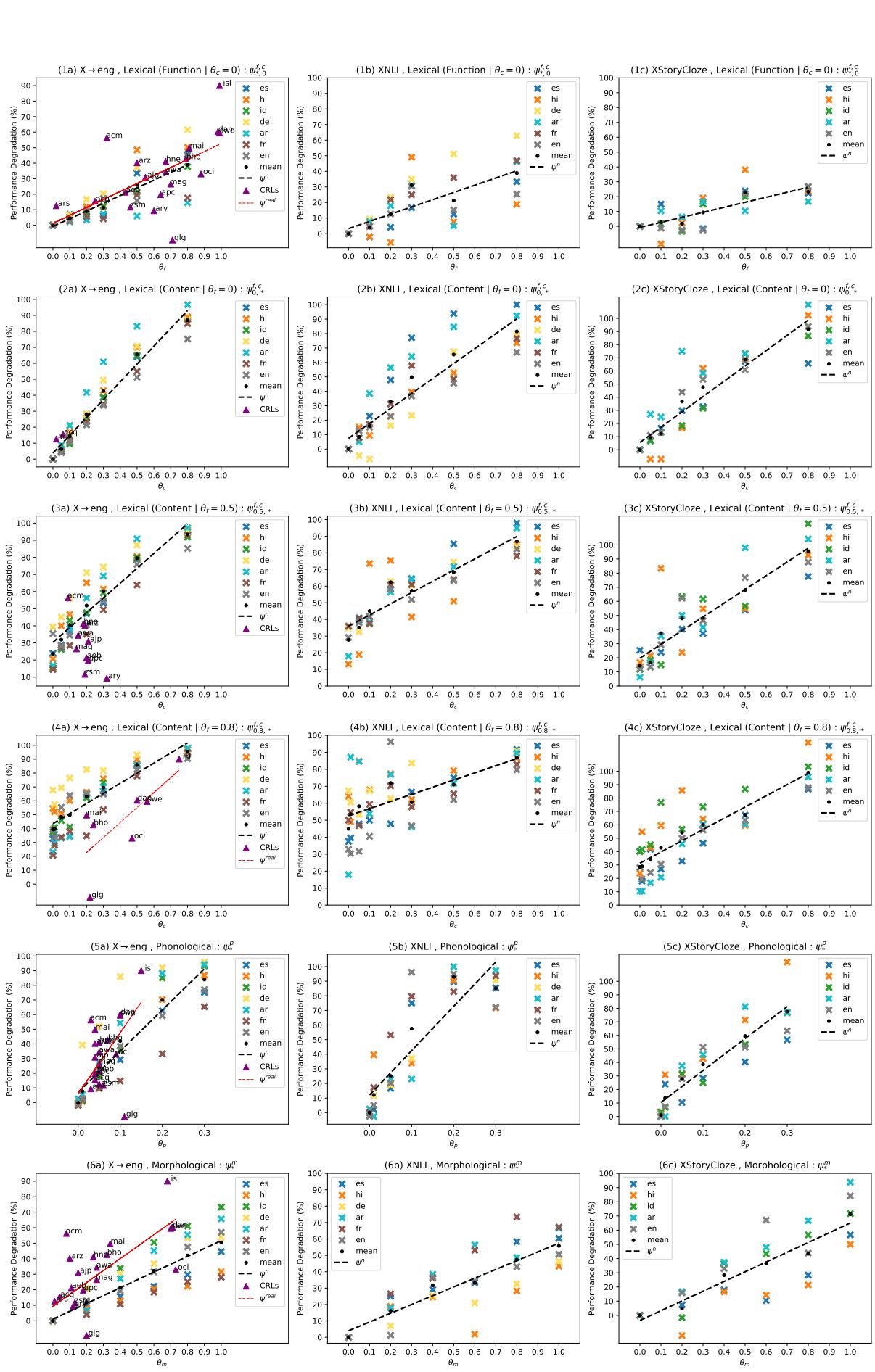
Let’s break down the insights from Figure 2 above:
- Phonological Noise (Row 3 - \(\phi^p\)): Look at the steep slopes. The model is incredibly sensitive to sound/spelling changes. Even a small amount of phonological noise (\(\theta_p = 0.2\)) causes massive performance degradation. This suggests that LLMs rely heavily on exact sub-word matching.
- Morphological Noise (Row 2 - \(\phi^m\)): These lines are much flatter. The model is surprisingly robust here. Even if you corrupt 50-80% of the suffixes, the model can still figure out the meaning based on the word stems.
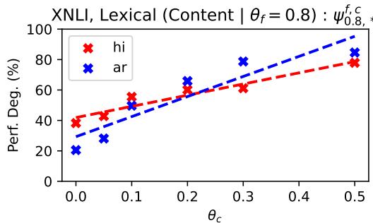
- Lexical Noise (Row 1 - \(\phi^{f,c}\)):
- Content vs. Function: The solid lines (where content words are changed) show steep degradation. Losing the nouns and verbs destroys understanding.
- Function Words: The impact of changing function words (like “the” or “of”) is lower than changing content words.
Result 2: Real Languages Follow Artificial Trends
Look closely at the scatter plots in Figure 2 again. You will see colored points (triangles and circles) scattered around the lines.
These points represent real CRL-HRLN pairs (e.g., the distance between Spanish and Galician, or German and Danish).
- The x-axis position is determined by the calculated \(\theta\) (the real linguistic distance).
- The y-axis is the actual Performance Degradation of the LLM on that real language.
The finding: The real languages mostly hug the trend lines generated by the artificial languages. This validates the entire methodology. It means we can accurately predict how badly an LLM will fail on a real dialect just by measuring its linguistic distance from the training language, without needing a labeled test set for that dialect.
Result 3: Comparing Languages and Tasks
Not all languages behave the same way. In Figure 3 below, we see the mean PD for different languages.
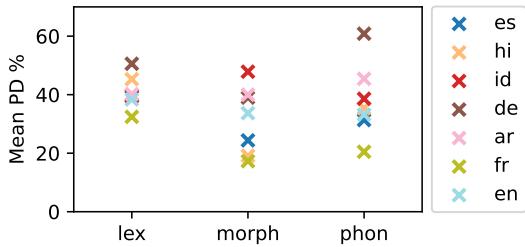
German (brown ‘x’) consistently suffers high degradation, especially with lexical noise. This might be due to how German compounds words—changing one component breaks the whole word. Conversely, Spanish (blue ‘x’) seems more robust.
The authors also noted that Translation (X \(\rightarrow\) eng) is a more stable task than classification (XNLI). In translation, if one word is corrupted, the model might still translate the rest of the sentence. In classification, corrupting a single key word can flip the logic of the entire premise, causing the model to crash to random guessing.
Result 4: The Composition of Noise
Real languages don’t just have one type of noise; they have all of them simultaneously. How do they interact?
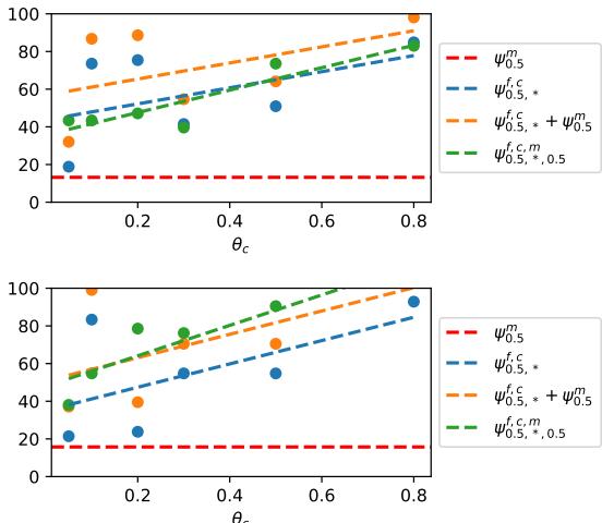
Figure 7 shows the effect of combining Lexical and Morphological noise.
- The Orange Line represents the theoretical sum of the two noises.
- The Green/Blue Lines show the actual experimental result.
Interestingly, the combined effect is not additive. As lexical noise increases (x-axis), it dominates the performance drop. If a word is completely replaced (lexical noise), it doesn’t matter if its suffix was also changed (morphological noise). The model is already broken on that word. This “overwrite” effect is a crucial insight for modeling real-world language variation.
Qualitative Analysis: How does the model break?
It is helpful to look at how the model fails when faced with these noises. The authors provide a detailed breakdown of error types.
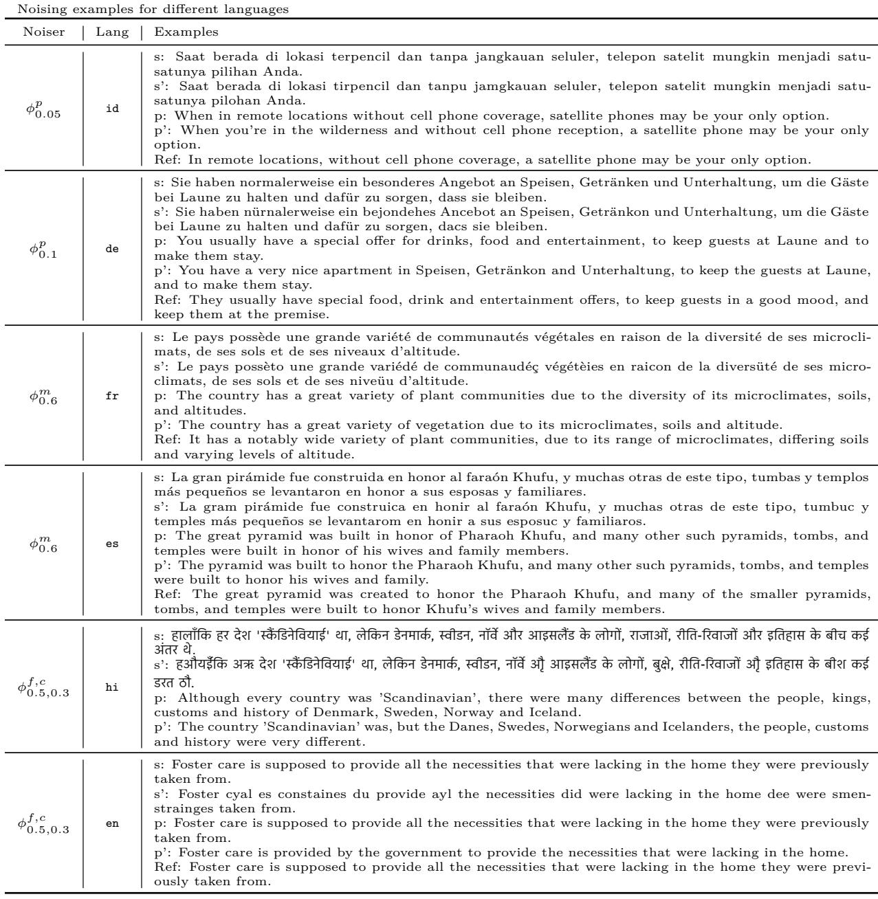
In Table 6, we can see specific examples:
- Phonological (\(\phi^p\)): In the Indonesian example (top row), a few vowel shifts cause the model to output specific English translations, but they are slightly degraded.
- Lexical (\(\phi^{f,c}\)): In the Hindi example, replacing content words causes the model to lose the specific subject (Danes, Swedes) and retreat to generic terms or completely different meanings.
Table 7 (below) provides a taxonomy of these errors for Spanish.
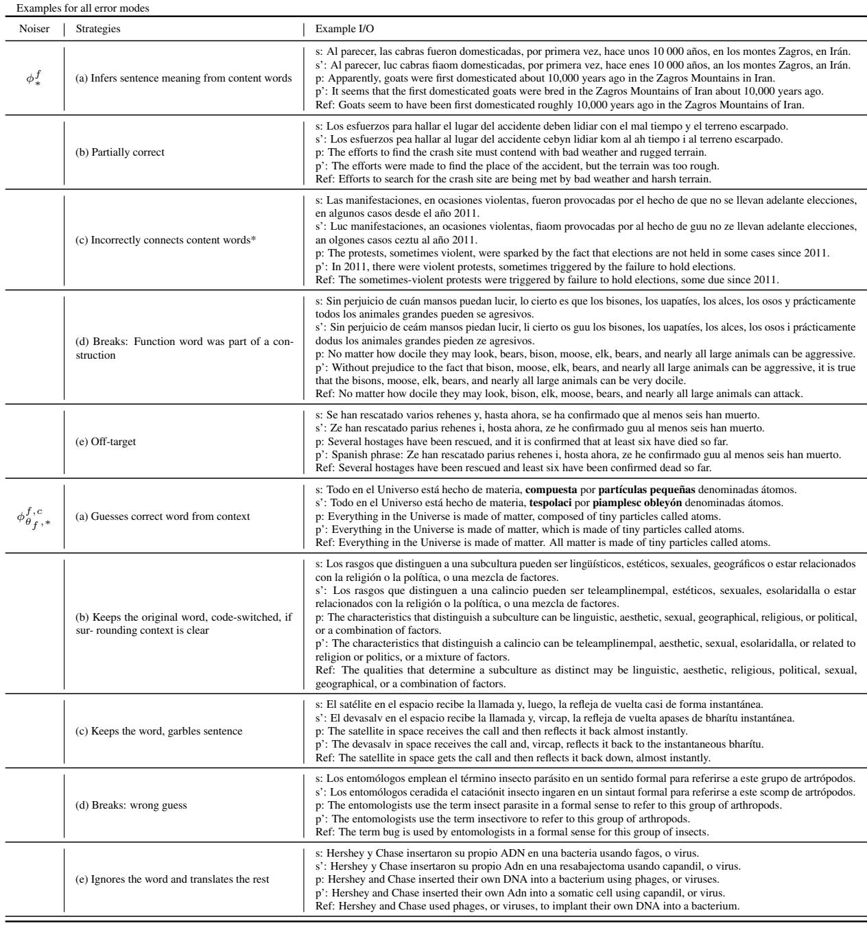
Notice row (d) under \(\phi^f\): “Breaks: Function word was part of a construction.” When the noise hits a function word that is grammatically necessary (like “sin” in “sin perjuicio”), the model’s understanding of the sentence structure collapses, even if the content words are intact.
Conclusion and Implications
This research bridges a massive gap in Natural Language Processing. By successfully modeling linguistic variation as noise, the authors have given us a tool to:
- Diagnose Failures: We can now say why an LLM fails on a dialect. Is it the spelling? The vocabulary? The grammar?
- Predict Performance: For the thousands of low-resource languages that have no test sets, we can simply calculate their distance (\(\theta\)) from a high-resource neighbor and look up the expected performance on the curves generated in this paper.
- Design Better Models: Knowing that models are hypersensitive to phonological noise (spelling/sound changes) suggests that we need better tokenizers or pre-training objectives that are robust to character-level variation.
The “Dialect Continuum” is vast, and LLMs have barely scratched the surface. Work like this moves us away from binary thinking (Does the model know Language X?) toward a nuanced understanding of language capabilities (How robust is the model to variation \(\theta\)?).
As we look toward a future of truly multilingual AI, simulating the evolution of language might just be the key to understanding it.