Stop Blending Data: Why Editing Model Weights is the Future of Multi-Task LLMs

If you have ever tried to train a Large Language Model (LLM) to be a “jack of all trades,” you know the struggle. You want a model that can solve math problems, write Python code, chat casually, and reason through logic puzzles.

The standard approach is Data Mixing. You take all your datasets—math, code, chat—throw them into a giant blender, and train the model on this mixed soup. The problem? It is incredibly expensive and notoriously difficult to tune. If you get the ratio of math-to-chat wrong, the model becomes great at algebra but forgets how to speak English. If you want to add a new skill later, you often have to re-blend and re-train from scratch.

But what if you didn’t have to mix the data at all? What if you could train a model on math, train a separate copy on code, and then just… add the skills together using simple arithmetic?

This is the premise of a fascinating new paper titled “DEM: Distribution Edited Model for Training with Mixed Data Distributions.” The researchers propose a method that is 11x cheaper than traditional training and yields significantly better performance on benchmarks like MMLU and BBH.

In this post, we will deconstruct how the Distribution Edited Model (DEM) works, the math behind “editing” model weights, and why this modular approach might be the future of LLM fine-tuning.

The Problem: The High Cost of the “Blender” Approach

To understand why DEM is necessary, we first need to look at the status quo: Multi-Task Instruction Fine-Tuning.

When creating a generalist assistant, engineers collect diverse datasets (\(D_1, D_2, \dots, D_n\)). One dataset might be Chain-of-Thought (CoT) reasoning, another might be dialogue.

In the standard Data Mixing approach, the objective is to learn a joint distribution that spans all these datasets. The training process samples batches from each dataset according to specific weights (e.g., 30% math, 50% chat, 20% logic).

This creates two massive headaches:

1. The Hyperparameter Nightmare: You have to find the perfect mixing weights. This requires training multiple proxy models or running expensive grid searches.
2. Rigidity: If you finish training and realize you forgot a specific coding dataset, you cannot simply “patch” it in. You effectively have to re-mix and re-train.

The researchers argue that we are making this too hard on ourselves. Instead of forcing the model to learn everything at once, we should let it learn skills individually and combine them later.

The Solution: Distribution Edited Model (DEM)

The core idea of DEM is modularity. Instead of mixing the data, we mix the models.

The process works in three distinct steps:

1. Independent Fine-Tuning: Take your base model (\(\Theta\)) and fine-tune it separately on each dataset (\(D_i\)) to create specific models (\(\Theta_{D_i}\)).
2. Extracting Distribution Vectors: Calculate the difference between the fine-tuned model and the base model. This difference represents the “skill” or “distribution” learned.
3. Vector Combination: Add these weighted differences back to the base model.

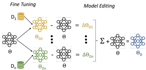
As shown in Figure 1, the architecture allows for a “plug-and-play” approach. You can train a “Math Model” and a “Chat Model” on different days, on different GPUs, and combine them later without ever letting the raw data touch.

Step 1: The Mathematics of Model Editing

Let’s look at the math, which is surprisingly elegant in its simplicity.

First, for every dataset \(D_i\), we obtain a fine-tuned model \(\Theta_{D_i}\). We then calculate a Distribution Vector (DV), denoted as \(\Delta \Theta_{D_i}\). This vector represents exactly how the weights shifted to learn that specific task.

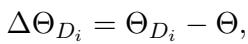
This operation is done element-wise. If a specific weight in the base model was \(0.5\) and the fine-tuned model changed it to \(0.7\), the distribution vector at that position is \(0.2\).

Step 2: The Mixing Recipe

Once we have these vectors—which we can think of as “skill modules”—we can combine them. The final Distribution Edited Model (\(\Theta_D\)) is created by adding a weighted sum of these vectors back to the original base model.

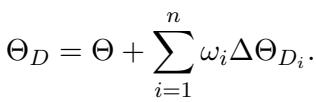
Here, \(\omega_i\) represents the weight (importance) of that specific distribution.

This is a crucial advantage: Tuning \(\omega_i\) is cheap. In the old “blender” method, if you wanted to change the weight of the math dataset, you had to re-train the model. In DEM, you just change the value of \(\omega_i\) in the equation above and essentially “slide” the model towards better math performance instantly. No gradient descent required.

Alternative: Model Interpolation

The authors also discuss a slight variation called Model Interpolation, where you simply take a weighted average of the fine-tuned models directly.

While this equation (Eq 3) looks similar, the authors found that the Distribution Vector method (Eq 2) provides more flexibility. Equation 2 allows the model to move “further” in the direction of a task than any single fine-tuned model did, effectively amplifying desirable traits.

Why is DEM So Much Cheaper?

The efficiency gains here are massive. Let’s break down the computational cost (\(c\)).

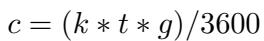
In a standard Data Mixing scenario, finding the optimal mix requires training many full models. If you have \(n\) datasets and want to try \(m\) different weight combinations, the complexity explodes.

With DEM, you train \(n\) models (one per dataset). The combination step happens post-training. You only need to run validation loops to find the best \(\omega\) weights.

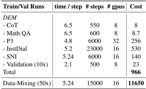
The results in Table 8 are staggering.

• DEM Total Cost: 966 GPU-hours.
• Data Mixing Cost: 11,650 GPU-hours.

DEM is roughly 11 times cheaper to produce. This democratizes the creation of robust, multi-task models, as it no longer requires the massive compute infrastructure needed to search for optimal data mixtures.

Experimental Results: Does It Actually Work?

Being cheap is good, but only if the model performs well. The researchers tested DEM using OpenLLaMA (7B) as the base, fine-tuning on diverse datasets including:

• P3: A massive collection of prompted tasks.
• Super Natural Instructions (SNI): 1,616 diverse NLP tasks.
• Chain of Thought (CoT): Reasoning tasks.
• MathQA: Math word problems.
• InstructDial: Dialogue tasks.

Downstream Performance

They evaluated the models on benchmarks like MMLU (knowledge), BBH (reasoning), and DROP (reading comprehension).

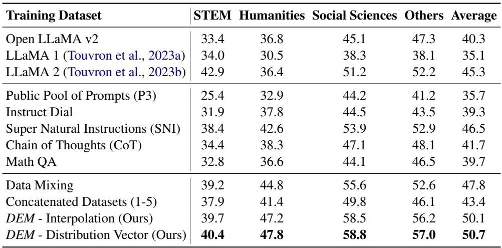
Table 11 highlights the dominance of DEM.

• OpenLLaMA Base: 40.3% average on MMLU.
• Data Mixing (The expensive baseline): 47.8%.
• DEM (Distribution Vector): 50.7%.

Not only did DEM beat the base model (which is expected), but it also beat the highly-tuned Data Mixing baseline by nearly 3 percentage points on MMLU. This pattern held true across other benchmarks as well.

HELM Evaluation

The researchers also ran the Hollistic Evaluation of Language Models (HELM), a rigorous standard for checking diverse capabilities.

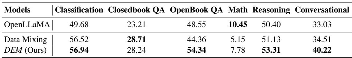
As shown in Table 3, DEM outperformed Data Mixing in Classification, OpenBook QA, Reasoning, and Conversational tasks. This proves that “stitching” models together via vector arithmetic doesn’t result in a “Frankenstein” model; it results in a coherent, capable generalist.

Does it Scale?

One common question in LLM research is: “Does this only work for small models?” The authors tested DEM on 3B, 7B, and 13B parameter models.

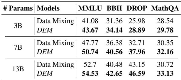
Table 4 confirms that the technique scales. Whether at 3B or 13B, DEM consistently outperforms Data Mixing. For example, on the 13B model, DEM achieves a 46.59 score on DROP compared to 43.15 for Data Mixing.

Why Does This Work? A Deep Dive

It feels counter-intuitive that simply adding weights together works so well. Why don’t the “Math weights” overwrite the “Chat weights” and ruin the model?

The researchers performed an exhaustive analysis to answer this, focusing on the geometry of the vectors.

1. Orthogonality of Tasks

They calculated the Cosine Similarity between the Distribution Vectors of the different datasets.

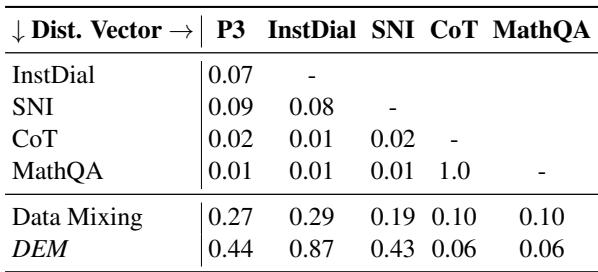
Table 7 reveals a fascinating property: Most Distribution Vectors are nearly orthogonal (similarity \(\approx 0\)).

• The vector for CoT (Reasoning) has almost zero overlap with InstructDial (Chat).
• MathQA is distinct from SNI.

This means that learning math moves the model’s weights in a completely different direction than learning dialogue. Because these vectors point in different directions in the high-dimensional parameter space, you can add them together without them interfering with each other. This is the mathematical reason why the model doesn’t “forget” how to chat when you add the math module.

2. Task Separation

To visualize this, the authors plotted the data using t-SNE, a technique for visualizing high-dimensional clusters.

Figure 2 visually confirms the cosine similarity data. The datasets form distinct, separate clusters (with some slight overlap between CoT and MathQA). This separation suggests that the “skills” required for these tasks rely on different features, enabling the vector addition strategy to work cleanly.

3. Layer-Wise Analysis

Where do these “edits” actually happen? The authors analyzed the Euclidean distance between the base model and the fine-tuned models layer by layer.

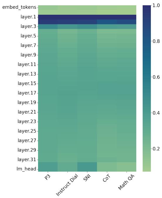
Figure 3 shows something surprising. Most of the heavy lifting happens in the first few layers (the darker regions at the top of the heatmap). The later layers remain relatively stable. This suggests that fine-tuning primarily adapts how the model processes and embeds basic features, rather than rewriting the deep reasoning circuits found in the middle/late layers. This localization of changes might be another reason why merging models is so non-destructive.

The Power of Incremental Learning

One of the strongest arguments for DEM isn’t just performance—it’s flexibility.

In a traditional pipeline, if you want to improve your model’s math score, you have to start the massive training run all over again with more math data. With DEM, you can simply:

1. Train a model on only the new math data.
2. Extract the vector.
3. Add it to your existing DEM.

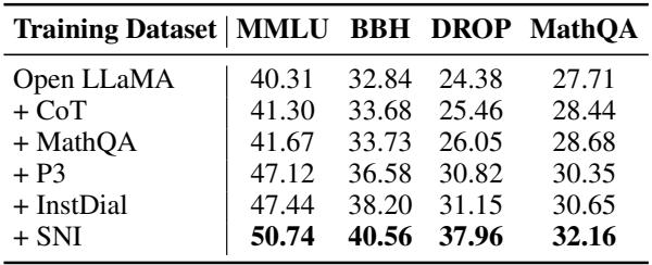
Table 5 demonstrates this capability. The authors started with the base model and progressively added vectors one by one (+CoT, +MathQA, +P3…). With every addition, the MMLU score ticked up. This allows for incremental upgrades, a feature that is critical for production environments where full re-training is too costly.

Conclusion

The “Distribution Edited Model” (DEM) paper challenges the assumption that LLMs must be trained on all data simultaneously to learn multiple tasks. By treating fine-tuned models as vectors in a parameter space, the authors demonstrated that we can perform arithmetic on “skills.”

Key Takeaways:

• Efficiency: DEM cuts training costs by over 90% compared to data mixing.
• Performance: It achieves higher scores on major benchmarks by allowing specialized optimization for each data source.
• Modularity: Tasks are largely orthogonal, allowing us to stack skills without catastrophic interference.

As we move toward larger models and more diverse datasets, the ability to “edit” models rather than “retrain” them will likely become a standard part of the AI engineer’s toolkit. DEM suggests a future where we don’t just train models; we compose them.