Introduction

The race for larger, more capable Large Language Models (LLMs) like Llama-3 and Mistral has led to incredible breakthroughs in artificial intelligence. However, this progress comes with a massive cost. As these models scale to billions of parameters, they become increasingly difficult to deploy in resource-limited environments. Running a 70-billion parameter model on a consumer-grade GPU—or worse, a mobile device—is often a non-starter due to memory and energy constraints.

To solve this, the AI community has turned to model compression. The two most common techniques are quantization (reducing the precision of the numbers, e.g., from 16-bit to 4-bit) and pruning (removing parameters entirely). While effective, these methods have drawbacks. Quantization often requires specific hardware support, and pruning—especially removing entire layers—is a destructive process. It’s like trying to make a book shorter by ripping out random chapters; you might save space, but you risk losing the plot.

But what if, instead of throwing away layers, we could merge them?

This is the core premise of a fascinating new paper titled “Pruning via Merging: Compressing LLMs via Manifold Alignment Based Layer Merging.” The researchers propose a novel method called MKA (Manifold-Based Knowledge Alignment). Instead of simply deleting redundant layers, MKA identifies layers that share similar “knowledge” and fuses them together. By utilizing advanced concepts like Manifold Learning and the Information Bottleneck (IB) principle, MKA achieves massive compression ratios with minimal performance loss.

In this post, we will walk through how MKA works, why it outperforms traditional pruning, and the math that makes it possible.

Background: The Redundancy of Giants

To understand why we can compress these models at all, we first need to understand the concept of overparameterization.

LLMs are trained on trillions of tokens, but they are also incredibly inefficient structures. Research suggests that modern deep neural networks are vastly overparameterized, meaning they have far more neurons and layers than are strictly necessary to solve the tasks they are trained for.

Mathematically, this redundancy implies that for a given model with parameters \(\theta\), there likely exists a smaller subset or a slightly different configuration \(\theta'\) that yields almost the same result.

As shown in the equation above, a subset of parameters is considered redundant if the difference in loss (error) between the original model and the modified model is negligible (\(\delta\)).

Traditional structured pruning tries to find and remove these redundant structures (like entire layers). However, simply removing a layer interrupts the flow of information. The network was trained to pass data sequentially; removing a step creates a “shock” to the system that often requires retraining to fix.

The authors of MKA ask a different question: Does the model learn similar representations at different layers? If Layer 20 and Layer 21 are doing almost the same thing, we shouldn’t delete one; we should combine them mathematically.

The MKA Framework

The Manifold-Based Knowledge Alignment (MKA) framework is built on two pillars:

1. Manifold Learning: To understand the geometry of the data flowing through the layers.
2. Layer Merging: Using Information Theory to fuse layers based on their similarity.

Figure 1 below provides a high-level overview of this architecture.

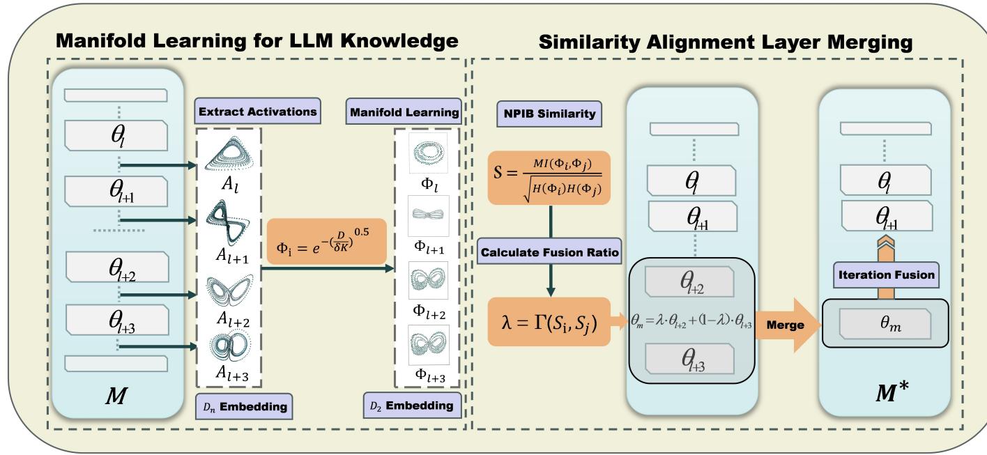
On the left, we see the extraction of activations and the creation of “manifolds.” On the right, we see the similarity analysis and the eventual merging of layers. Let’s break this down step-by-step.

Step 1: Manifold Learning and Diffusion Maps

A raw layer activation is just a massive matrix of numbers. Comparing two layers directly by looking at their weights or raw outputs is noisy and often inaccurate because they might be representing the same information in slightly different high-dimensional spaces.

To solve this, the authors rely on the Manifold Hypothesis. This hypothesis states that high-dimensional data (like LLM activations) actually lies on a much lower-dimensional structure (a manifold) embedded within that space. Think of a coiled spring; it exists in 3D space, but the data itself is essentially a 1D line curled up.

To capture this structure, MKA uses Diffusion Maps.

Constructing the Graph

First, for a specific layer \(l\), the method takes the activations \(H\) from a set of inputs. It constructs a graph where each node is an activation vector, and the connection between them is determined by how similar they are. This similarity is calculated using a Gaussian Kernel:

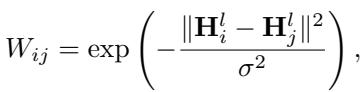
Here, \(W_{ij}\) represents the affinity (closeness) between two activation vectors. If they are close, the value is near 1; if far, near 0.

The Diffusion Operator

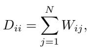
Next, we normalize this relationship to create a probability matrix. We calculate the “degree” of each node (the sum of its connections):

And use it to define the Diffusion Operator \(P\):

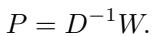
This operator \(P\) describes a “random walk” on the data. If you were standing on a data point and took a random step, \(P\) tells you where you are likely to land. This effectively captures the local geometry of the data manifold.

Creating the Embedding

Finally, to get a clean, low-dimensional representation of what the layer is actually knowing, the method performs spectral decomposition (eigen-decomposition) on this operator. The resulting Diffusion Map at time \(t\) is defined as:

This vector \(\Phi_t\) is a compressed, geometric fingerprint of the layer’s knowledge. If two layers produce similar diffusion maps, they are processing information in geometrically similar ways, even if their raw weights look different.

Step 2: Measuring Similarity with Mutual Information

Now that we have these clean manifold embeddings (\(\Psi^l\) for layer \(l\) and \(\Psi^m\) for layer \(m\)), we need a robust metric to compare them. The authors choose Mutual Information (MI).

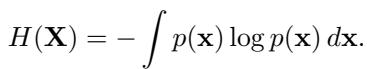
MI measures how much information one variable tells us about another. It is defined using entropy (\(H\)):

To make this practical for comparing layers, the authors utilize a Normalized Similarity Score (\(S_{lm}\)). This scales the mutual information so that values are comparable across different parts of the network:

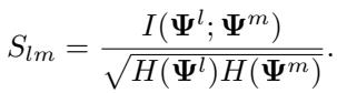
If \(S_{lm}\) is high, it means Layer \(l\) and Layer \(m\) are highly redundant—they “know” the same things. These are our candidates for merging.

Step 3: Layer Merging via Information Bottleneck

Once a pair of similar layers is identified (e.g., Layer 31 and Layer 32), we merge them into a single layer. But we don’t just take a simple average (\(\frac{Layer A + Layer B}{2}\)). We want to preserve the most critical information.

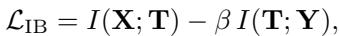
The authors employ the Information Bottleneck (IB) principle. The goal of IB is to find a compressed representation \(T\) of input \(X\) that keeps as much information as possible about the target \(Y\).

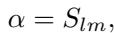
In the context of layer merging, the method seeks a merged representation \(\Psi^c\) that retains the shared information of the original two layers while filtering out noise. The merging is modeled as a linear combination weighted by a parameter \(\alpha\):

The crucial part is determining \(\alpha\) (the merging ratio). While the paper derives a complex derivative for the optimal \(\alpha\), they find that a heuristic approximation works efficiently and effectively. They set \(\alpha\) proportional to the similarity score:

Finally, the weights of the new merged layer \(\theta_c\) are calculated:

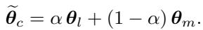
This results in a compressed model where two layers have mathematically become one, ideally retaining the capabilities of both.

Experiments and Results

The theory sounds solid, but does it work in practice? The researchers tested MKA on several popular open-source models, including Llama-2 (7B, 13B), Llama-3 (8B), and Mistral-7B.

MKA vs. Traditional Pruning

The primary comparison was against state-of-the-art structured pruning methods like ShortGPT, SLEB, and PruneMe. The metric? Accuracy on the massive MMLU benchmark.

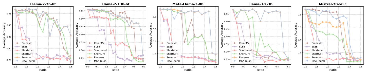
The graph above tells a compelling story. The X-axis represents the pruning ratio (how much of the model was removed), and the Y-axis is accuracy.

• Look at the Blue Line (MKA): It consistently stays higher than the other methods (green, orange, red) as the compression ratio increases.
• Stability: While other methods see a sharp “collapse” in performance when pruning exceeds 20-30%, MKA maintains respectable accuracy even at compression ratios approaching 40-50%.
• Llama-2-13B: MKA achieves nearly a 58% compression ratio on this model while keeping the performance relatively stable, which is a massive reduction in size.

Combining Merging with Quantization

One of the most exciting findings is that MKA isn’t mutually exclusive with quantization. You can merge layers and reduce bit precision.

Table 1 below shows the results of combining MKA with quantization methods like SmoothQuant, GPTQ, and AWQ.

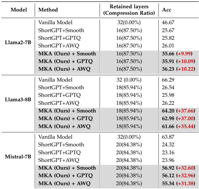
The difference is stark. When compressing Llama-3-8B to roughly 15% of its original size (retained layers + quantization), standard pruning (ShortGPT) drops to ~26% accuracy. MKA with SmoothQuant maintains 64.20% accuracy. That is the difference between a broken model and a usable one.

Visualizing the Similarity

Why does this work? We can look at the similarity matrices generated by the manifold learning process.

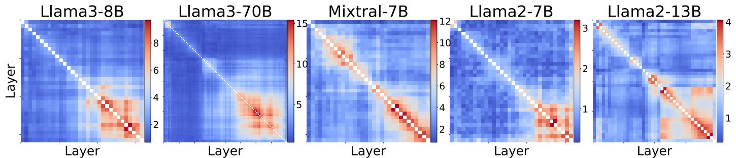
These heatmaps show the similarity between layers. The bright blocks in the bottom right of the matrices (representing the deeper layers of the network) indicate high similarity.

• Interpretation: This confirms that deep layers in LLMs are highly redundant. They are refining the same representations over and over.
• The “Collapse”: Notice the earlier layers (top left) are less similar. This explains why merging usually targets the later stages of the model; the early layers are doing distinct, foundational work (like feature extraction) that cannot be easily merged.

The Importance of Iteration

MKA uses an iterative approach—merge a pair, recalculate, merge another pair. The authors compared this to a “one-shot” approach where all merges happen at once.

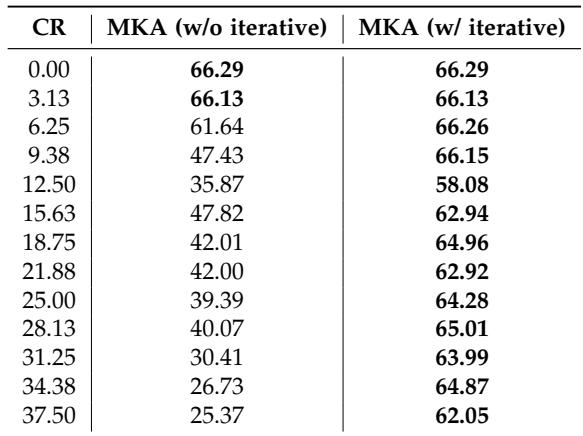
As shown in Table 4, the iterative approach (right column) is vastly superior. At a 37.5% compression ratio, the non-iterative approach crashes to 25% accuracy, while the iterative MKA holds strong at 62%. This suggests that when layers are merged, the manifold structure changes slightly, requiring a re-evaluation of the network’s geometry before the next merge.

Discussion: Why This Matters

The implications of MKA extend beyond just making files smaller.

Robustness Across Subjects

The researchers broke down performance by subject on the MMLU dataset.

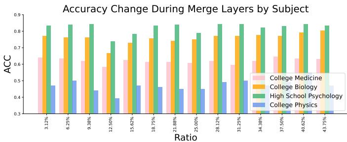
Interestingly, not all knowledge is impacted equally.

• High School Psychology (Green): Extremely robust. You can compress the model significantly without losing performance here.
• College Physics (Blue): Very sensitive. Performance fluctuates wildly. This suggests that “reasoning-heavy” tasks might rely on specific, delicate circuits in the model that are more susceptible to merging artifacts than general knowledge tasks.

Universality

The authors also applied MKA to Mixture-of-Experts (MoE) models like Mixtral and hybrid architectures like Jamba.

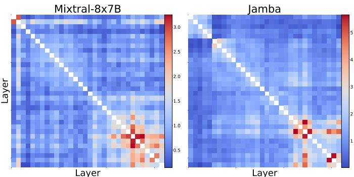
The similarity matrices (Fig 4) look different—notice the cross-patterns in Mixtral. This indicates that MoE models handle redundancy differently, likely due to their routed expert architecture. However, the presence of high-similarity regions suggests MKA can be adapted for these next-gen architectures as well.

Why Manifold Learning?

Finally, the authors justified their complex “Manifold” approach over simpler metrics like Euclidean distance or Cosine similarity.

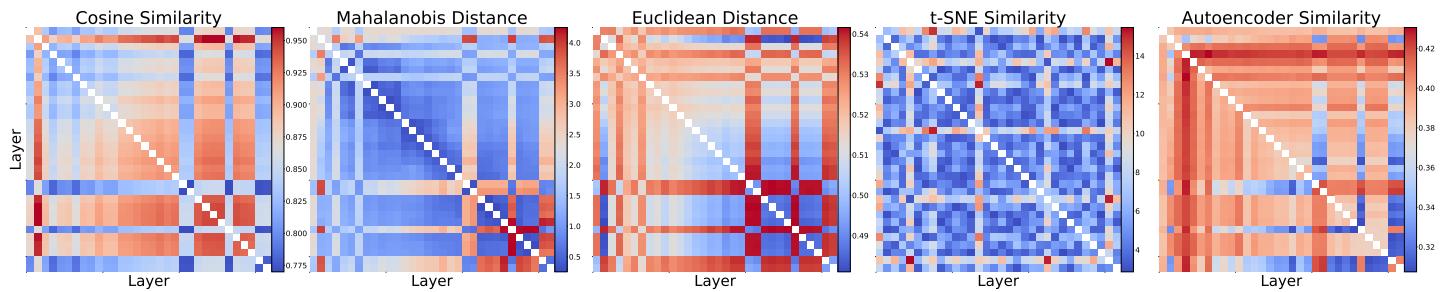
Figure 5 compares different similarity metrics. Simple metrics like Cosine Similarity (far left) show everything as somewhat similar (lots of red), which leads to “false positives”—merging layers that shouldn’t be merged. The Manifold-based similarity provides a cleaner, more structural view of the data, allowing for precise surgical merges rather than blunt force combinations.

Conclusion

The paper “Pruning via Merging” presents a compelling step forward for Efficient AI. By shifting the paradigm from subtraction (pruning) to integration (merging), MKA preserves the dense web of knowledge that LLMs spend weeks learning.

The key takeaways are:

1. Redundancy is Geometric: Layers are redundant not just in weights, but in the shape (manifold) of their activations.
2. Merge, Don’t Delete: Fusing layers using Information Theory preserves performance far better than removing them.
3. Synergy: MKA works alongside quantization, unlocking massive compression ratios (over 40-50%) that could bring powerful LLMs to laptops and phones.

As models continue to grow, techniques like MKA will be essential—not just for saving hard drive space, but for making AI accessible, sustainable, and efficient for everyone.