](https://deep-paper.org/en/paper/2407.02646/images/cover.png)
Why do language models sometimes behave like geniuses and other times like mysterious black boxes? Mechanistic Interpretability (MI) is the attempt to answer that question by reverse-engineering what these models actually compute—down to neurons, attention heads, and the circuits that connect them. This article distills a recent survey, “A Practical Review of Mechanistic Interpretability for Transformer-Based Language Models,” into a hands-on, task-centered guide for students and practitioners who want to move from curiosity to reproducible investigations.
What you’ll get from this guide
- A compact transformer refresher so you’re fluent in the language of MI.
- The three core objects MI studies (features, circuits, universality), and why each matters.
- The principal techniques (logit lens, intervention/patching, sparse autoencoders, probing, visualization), how they’re used, and their limitations.
- A step-by-step, task-centric “Beginner’s Roadmap” for feature, circuit, and universality studies.
- Concrete examples, evaluation tips, and an honest discussion about open problems and where research should go next.
If your goal is to run your first interpretability experiment or to read papers with more clarity about their methods and claims, this walkthrough will help you do that confidently.
1. Quick transformer primer (so MI speaks your language)
Transformers process token sequences by maintaining a vector representation for each token and iteratively refining it layer by layer. The residual stream is the sequence of these representations across layers.
A compact view of the layer update:
- Let \(h_i^l\) be the representation for token position \(i\) at layer \(l\).
- Each layer contributes an attention output \(a_i^l\) and a feed-forward output \(f_i^l\).
- The residual update is commonly written as: \[ h_i^l = h_i^{l-1} + a_i^l + f_i^l. \]
Multi-head attention (MHA) lets each token incorporate information from other positions via learned query/key/value projections. The feed-forward (FF) sublayers are per-token MLPs that often encode and produce features used later in the model. The unembedding \(W_U\) maps final-layer representations to logits over the vocabulary.
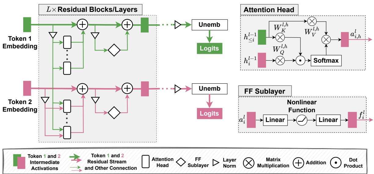
Figure 1: Architecture of transformer-based LMs — tokens flow through residual streams, attention heads, and FF sublayers before being projected via the unembedding to logits.
2. What is Mechanistic Interpretability (MI)?
At its core, MI attempts to “open the hood” and describe the internal computations of a model in human-understandable algorithmic terms. Instead of just asking “what output did the model give?”, MI asks “how did the model compute that output?”
The MI community often organizes analyses around three fundamental objects:
- Features — What atomic, human-interpretable inputs or concepts are encoded in model activations?
- Circuits — How do model components (neurons, heads, FF blocks) interact to implement specific behaviors or algorithms?
- Universality — Do the same features and circuits appear across different models, initializations, sizes, or tasks?
These three questions guide most MI investigations and form the basis of the task-centric roadmap we’ll present later.
3. Fundamental objects of MI (with examples)
Features
A feature is some interpretable property encoded in activations—e.g., “is French text”, “an entity name”, or an arithmetic indicator. Features can be localized to single neurons, directions in activation space, or distributed subspaces.
Circuits
A circuit is a subgraph of the model (nodes and edges) that implements a behavior. For example, Elhage et al. discovered a small induction circuit in a toy model: one head detects a prior occurrence, another uses that signal to copy tokens forward.
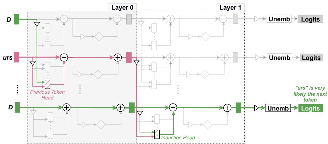
Figure 2: An induction circuit that detects and continues repeated subsequences by linking a previous-token-detection head and an induction head.
Universality
If we discover a circuit in GPT-2 small, does a similar circuit exist in Gemma or Llama? Universality studies ask how much transfer or convergence there is across models and tasks. Mixed experimental findings show some components (like induction heads) recur, while some circuits are sensitive to initialization and training details.
4. The MI toolbox — core techniques and what they tell you
Below are the most-used techniques in MI, how they work at a high level, and practical considerations when applying them.
4.1 Vocabulary projection methods (Logit Lens and variants)
Idea: take an intermediate activation (e.g., \(h_i^l\)), apply the model’s unembedding \(W_U\) (often with some alignment), and inspect the resulting logits. This gives a vocabulary-based “what the model is thinking at this layer” signal.
Why use it
- Gives a human-readable window into intermediate predictions.
- Good for hypothesis generation: which tokens a layer is favoring.
Practical caveats
- Early layers may not sit in the same basis as the final layer; raw projection can be misleading.
- Tuned lenses or learned linear translators (e.g., Tuned Lens) often improve fidelity.
- Projections decode token probabilities, so they’re limited to features expressible in the vocabulary space.
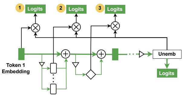
Figure 4: Logit lens implementation showing RS, attention head outputs, and FF sublayer projections.
Key variants and extensions
- Tuned Lens / Attention Lens: learn small translators from intermediate activations into the final-layer basis.
- Future Lens / Patchscope: combine projection with intervention to decode information about future tokens or other latent features.
4.2 Intervention-based methods (activation patching / causal tracing)
Idea: treat the model as a computational/causal graph. Run three inferences—clean, corrupt, and a patched run—and measure how replacing parts of the activation affects outputs. Interventions can be:
- Noising-based (ablation): remove a component’s contribution.
- Denoising-based (causal patching): restore a component’s clean contribution in a corrupt run.
Why use it
- Provides causal evidence of necessity / sufficiency for components in a behavior.
- Core technique for circuit localization.
Common workflow (practical)
- Run model on a clean input and cache activations.
- Run model on a corrupt input and cache activations.
- Patch activations from the corrupt run into the clean run (node patching) or along specific computational paths (edge / path patching).
- Measure changes in logits, logit differences, or full KL divergence.
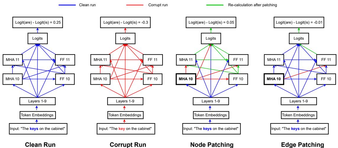
Figure 5: Example of node and edge patching illustrating how localized interventions pinpoint causal components (subject–verb agreement example).
Practical caveats
- Out-of-distribution (OOD) risk: replacing activations with arbitrary vectors may push the model into unrealistic states. Resampling/mean ablation reduce this risk.
- Granularity matters: whole-neuron patching assumes localist representations; subspace patching (DII/DAS) can reveal distributed encodings.
Representative developments
- Activation patching & path patching (faithful but compute-heavy).
- ACDC, EAP, EAP-IG (automated and more scalable approaches to localize edges/nodes).
- Patchscope: patch activations into a target LM + prompt to decode what a representation represents.
4.3 Sparse Autoencoders (SAEs)
Problem they address: superposition — models pack more features than they have neurons, producing polysemantic neurons.
Idea: train an autoencoder that maps a model activation \(h\in\mathbb{R}^d\) into a higher-dimensional sparse vector \(f(h)\in\mathbb{R}^s\) with \(s>d\), then decode back to reconstruct \(h\). A sparsity penalty encourages monosemantic units.
Typical SAE training loss:
\[ \mathcal{L}(h,\hat h) = \frac{1}{|\mathcal{X}|}\sum_{X\in\mathcal{X}}\Big(\|h(X)-\hat h(X)\|_2^2 + \lambda \|f(h(X))\|_1\Big) \]Why use it
- Opens up features that were previously entangled in superposition.
- Supports open-ended feature discovery by producing a dictionary of candidate features.
Practical caveats
- The sparsity–reconstruction trade-off is real; high sparsity can reduce reconstruction fidelity.
- Evaluating interpretability requires human labeling or LLM-based scoring; SAE features may or may not be functionally used by the model.
- New SAE variants (TopK, JumpReLU, Gated SAE, Matryoshka) attempt to improve the sparsity–fidelity balance or discover hierarchical features.
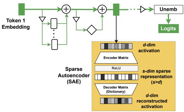
Figure 6: SAE architecture showing encoder → sparse s-dim representation → decoder back to d-dim reconstruction.
4.4 Probing and visualization (essential but limited)
- Probing: train a classifier (often linear) on activations to detect a pre-defined property. It’s quick and informative but correlational.
- Visualization tools: attention heatmaps, token highlights, and dashboards (e.g., CircuitsVis, Neuronpedia) help form hypotheses but must be validated with causal methods.
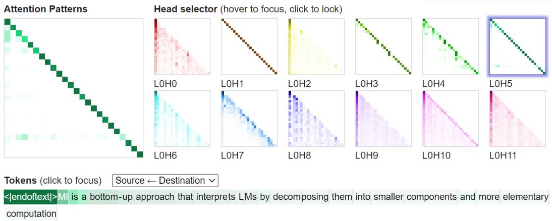
Figure 8: Example attention visualization interface showing different heads and their attention patterns.
A compact summary of these techniques and trade-offs is available in Table 2 (survey figure).
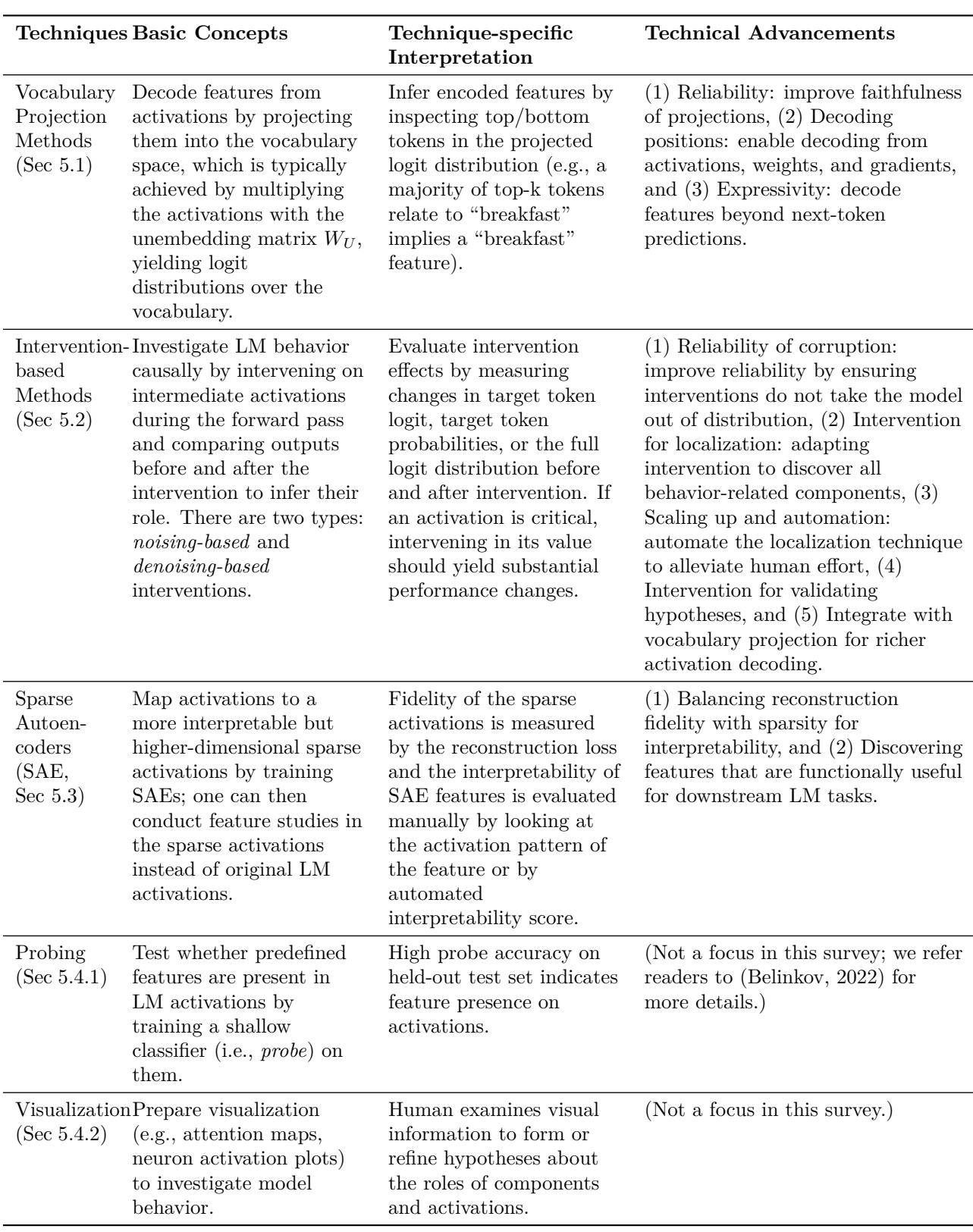
Figure (table): Techniques overview—logit lens, interventions, SAEs, probing, and visualization with their strengths and limitations.
5. A beginner’s, task-centric roadmap to MI
The survey’s central practical contribution is a “Beginner’s Roadmap” that organizes MI research by task (feature study, circuit study, universality) and gives actionable workflows for each. Below are condensed, step-by-step recipes you can follow.
5.1 Feature study — two paths
Feature studies ask: “What does this activation encode?”
Path A — Targeted feature study (you have a hypothesis)
- Hypothesis generation: pick a specific feature (e.g., “is_python_code”, “contains person name”).
- Hypothesis verification:
- Probing (train a probe) — works well if you have labeled data.
- PatchScope / DII / DAS — use when you suspect the feature lives in a subspace or when you want causal evidence.
- Evaluation: probe accuracy, intervention effect sizes, or DAS alignment metrics. Remember probes are correlational—use patching for causal claims.
Path B — Open-ended feature discovery (you don’t know what to expect)
- Observe:
- Use logit lens / tuned lens to see candidate tokens a representation promotes.
- Visualize neuron or SAE feature activations to collect highly activating contexts.
- Train SAEs to extract candidate monosemantic features.
- Explain:
- Human annotators or LLMs (as explainers) map intermediate explanations to natural-language descriptions. Combine approaches: have an LLM propose labels and humans verify.
- Evaluate:
- Faithfulness: reconstruction loss, patching/steering experiments (does manipulating the feature change outputs?), probe performance.
- Interpretability: human ratings or LLM-scored explanation consistency.
Interfaces that help
- Early neuron labeling interfaces showed top activating snippets and promoted tokens (helpful to find base64 or language-specific neurons).
- Neuronpedia and SAE dashboards integrate many diagnostics (activation histograms, top tokens, steering tests, auto-generated explanations) to reduce manual effort.
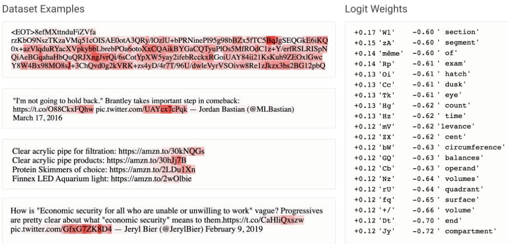
Figure 10: Visual interface demonstrating an example neuron that strongly activates for base64-like tokens.
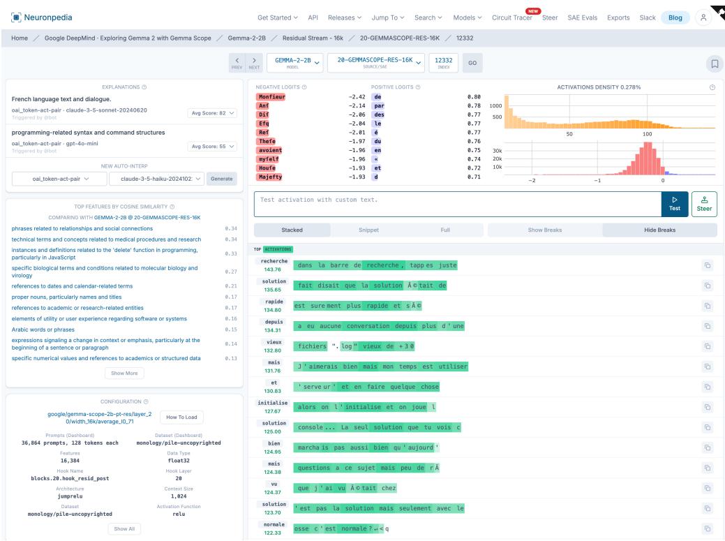
Figure 11: Neuronpedia-like dashboard for feature interpretation with auto-explanations and steering tests.
5.2 Circuit study — finding the pathway
Circuit studies ask: “Which subgraph implements this behavior, and how?”
- Choose a clear, reliable LM behavior (high accuracy on a dataset). Examples: IOI (indirect object), arithmetic, induction pattern completion.
- Define the computational graph:
- Decide nodes (attention heads, FF outputs, SAE features) and edges (residual stream connections). Choice of granularity affects interpretability and computational cost.
- Localization:
- Use activation patching and path patching to measure necessity/sufficiency.
- Use automated tools (ACDC, EAP-IG) if you need to scale search across many components.
- Interpretation:
- Generate hypotheses using visualization and vocabulary projection.
- Validate hypotheses with targeted interventions (e.g., does ablation remove a predicted effect?).
- Evaluation:
- Faithfulness: does the discovered subcircuit reproduce the behavior?
- Minimality: are the components necessary?
- Completeness: does the circuit cover all components contributing to the behavior under realistic perturbations?
Example: IOI circuit in GPT-2 small
- Define a position-dependent computational graph with attention heads as nodes.
- Localize with path patching and find “name mover heads” that copy the correct entity.
- Hypothesis validation: measure copy scores, use logit lens on OV outputs, and show high top-5 token recall for names—confirming the head’s copying function.
5.3 Universality study — how general are your findings?
Workflow:
- Define scope: features or circuits?
- Choose variation axes: model sizes, architectures, seeds, training data.
- Run feature/circuit studies across models and compare:
- Feature universality: compare activation vectors on a shared dataset (Pearson correlation for feature activations, nearest-neighbor matching across models).
- Circuit universality: check for functionally equivalent components and similar algorithms (e.g., do different models implement the same name mover pattern?).
- Evaluation: distributions of similarity scores, overlap metrics, and qualitative analyses of algorithmic equivalence.
Empirical notes
- Feature universality appears limited at the neuron level (1–5% of neurons may be “universal” across seeds), but SAE-derived features show more cross-model alignment in some studies.
- Some components (induction-style heads) recur often, while other circuits can be qualitatively different depending on initialization and training.
6. Case studies — translating the roadmap into experiments
Two representative examples from the literature show the roadmap in action.
- Targeted probing example (Gurnee et al.)
- Hypothesis: “is_french_text” appears in FF activations.
- Process: build labeled dataset → extract activations → train sparse probe with adaptive thresholding → evaluate with F1/precision/recall → iterate over layers and models to test universality.
- Open-ended SAE example (Bricken et al.)
- Hypothesis-free discovery on a toy model.
- Process: train SAE on activations → present SAE features in an interface with top activations, vocab projections, and steering → human annotators label features and score interpretability.
- IOI circuit example (Wang et al. 2022)
- Selected the IOI behavior → defined graph with attention heads (position-dependent) → localized nodes & edges with path patching → interpreted heads as name movers and inhibitors via attention patterns and logit-lens-style probes → validated and measured faithfulness/minimality.
7. Key findings from MI (what we’ve learned so far)
A short tour of recurring discoveries and themes:
- Neurons are often polysemantic; features are frequently distributed or superposed rather than neatly localised to single neurons.
- The superposition hypothesis: models can encode more features than they have neurons, using different linear combinations.
- SAEs can surface many monosemantic-looking features, but the faithfulness and functional importance of SAE features remain active research questions.
- Attention heads often acquire specialized roles (copying, induction, previous-token detection, suppression), and many circuits composed of heads+FFs are discoverable for specific tasks.
- FF sublayers frequently behave as key-value memories: the first matrix produces keys, the second stores values that are promoted to logits.
- Some structures (e.g., induction heads) appear repeatedly across models and scales; other circuits are sensitive to initialization and training details.
- Training dynamics: phase changes and grokking correspond to emergent circuitry formation in many settings.
- Applications include model steering, debiasing (ablate spurious features), and safety monitoring (detecting safety-relevant directions in latent space).
Tables of discovered neurons and circuits (selected examples) summarize these findings in the survey. See Table images in the survey for a compact listing.
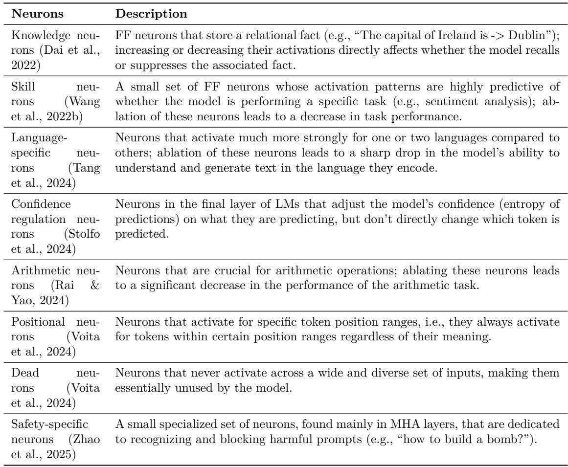
Figure 12: SAE feature interface showing diagnostics used to evaluate and label candidate features.
8. Evaluation, pitfalls, and best practices
Interpreting models is subtle; here are practical recommendations based on the survey’s synthesis and the community’s experience.
- Use causal methods to support causal claims. Probes indicate presence, but interventions show use.
- Beware of OOD effects when patching activations—resampling ablations and mean ablations reduce this risk compared to zero or random ablation.
- Choose your computational graph granularity deliberately—coarse graphs (component-per-layer) are cheaper but may miss position-dependent behavior; fine granularity reveals more detail at higher cost.
- Combine techniques: use vocabulary projection + interventions + SAEs to triangulate interpretations and reduce false positives.
- Automate where possible: EAP-IG and ACDC-style methods speed localization, but always sanity-check automated outputs with causal tests.
- Evaluate interpretability along two axes: faithfulness (does the discovered mechanism causally drive behavior?) and intelligibility (can humans reliably label and reason about it?).
- Use synthetic benchmarks (like Tracr) to validate your toolchain, but validate on naturally-trained models too—synthetic success does not guarantee real-world generality.
9. Open challenges and promising directions
The MI survey surfaces a set of open problems that are both technically compelling and practically important:
- Scalability: How do we scale faithful circuit discovery and SAE training to billion-parameter LLMs without massive compute?
- Automation of hypothesis generation: Human intuition currently drives much of the exploration; semi-automated hypothesis generation with human-in-the-loop reviewers could accelerate discovery.
- Faithful evaluation: Benchmarks (e.g., Tracr, RAVEL, MIB, SAEBench) help, but we need better agreed-upon metrics for faithfulness, completeness, and interpretability that generalize to natural models.
- SAE limitations: Better architectures, hierarchical dictionaries (Matryoshka SAEs), and end-to-end training that link SAE detection to behavioral influence are promising.
- From features to propositions: Decoding higher-level propositions (e.g., “I support X”) rather than low-level attributes may better serve high-stakes safety work.
- Practical utility: Moving from descriptive discoveries to tools that improve model alignment, robustness, or model editing remains an active frontier.
10. Final practical checklist — start your own MI investigation
If you want to run an MI experiment this afternoon, here’s a compact checklist to get you from question to result.
- Pick a specific behavior (high-accuracy task) or a focused feature question.
- Choose a model and dataset that isolate the behavior.
- Decide your computational graph and granularity (heads, FFs, SAE features).
- Generate hypotheses via visualization, logit lens, or initial probing.
- Localize with causal interventions (node/edge patching, path patching). Automate with EAP-IG/ACDC if needed.
- Interpret components with vocab projections and targeted causal tests.
- Evaluate faithfulness (intervention restores behavior), minimality (are components necessary?), and completeness.
- Document: share datasets, scripts, and patching procedures. Reproducibility is paramount in interpretability.
Mechanistic interpretability has transformed from a set of exploratory techniques into a maturing, task-centered toolbox. The survey this article is drawn from is an excellent map to the territory: it doesn’t claim that all questions are solved, but it gives newcomers a structured path for asking good questions, choosing the right tools, and evaluating claims rigorously. If you’re a student, researcher, or practitioner who wants to understand, debug, or align language models, MI offers both the language and the methods to make the opaque a lot more transparent—one circuit at a time.