Introduction

In the world of computational science, simulating reality is a balancing act. Whether predicting the weather, designing aerodynamic cars, or modeling structural stress, scientists rely on Finite Element Methods (FEM). These methods break down complex physical shapes into a grid of small, simple shapes—triangles or tetrahedra—called a mesh.

The golden rule of FEM is simple: the more points (or nodes) you have in your mesh, the more accurate your simulation. However, more points mean significantly higher computational costs. A simulation that takes minutes on a coarse mesh might take weeks on a dense one.

This creates a fundamental problem: How do we achieve high accuracy without exploding the computational budget?

The answer lies in Mesh Adaptivity. Instead of uniformly increasing the number of points everywhere, we can move the existing points to concentrate them in areas where the simulation is most complex (like a shock wave or a turbulent eddy) and spread them out where nothing much is happening.

Today, we are diving into a groundbreaking paper titled “G-Adaptivity: optimised graph-based mesh relocation for finite element methods.” The authors propose a novel way to solve this problem using Graph Neural Networks (GNNs). Unlike previous machine learning attempts that try to mimic classical mathematical solvers, this approach learns to move mesh points by directly minimizing the simulation error.

Let’s look at the performance difference right away.

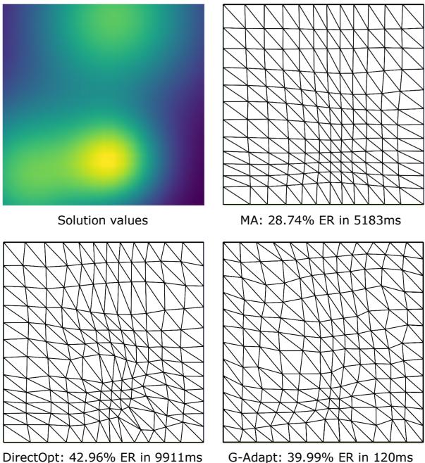
As shown above, the new method (G-Adapt) achieves error reduction comparable to the gold-standard mathematical approach (Monge-Ampère or MA) but runs at a fraction of the speed (120ms vs 5183ms).

In this post, we will unpack how G-Adaptivity works, why it prevents the common problem of “tangled” meshes, and how it performs on complex physics problems like Fluid Dynamics.

The Background: The Quest for the Perfect Mesh

To understand why G-Adaptivity is a big deal, we first need to understand the mathematical problem it solves.

The PDE Context

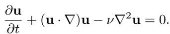
We are trying to solve Partial Differential Equations (PDEs). In abstract form, we are looking for a solution \(u\) for an equation like this:

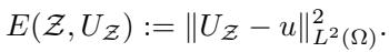
When we solve this numerically using FEM, we get an approximate solution \(U_{\mathcal{Z}}\). Our goal is to minimize the error between the real physics \(u\) and our approximation \(U_{\mathcal{Z}}\). This is usually measured as the squared \(L^2\)-error:

r-Adaptivity: Moving the Mesh

There are two main ways to adapt a mesh:

1. h-adaptivity: You cut existing triangles into smaller ones. This changes the number of points and the data structure, which can be computationally messy.
2. r-adaptivity (Relocation): You keep the number of points fixed but move their coordinates. This is the focus of this paper.

Classically, r-adaptivity is treated as a problem of “equidistribution.” Imagine you have a “monitor function” \(m(\mathbf{z})\) that tells you where the error is high. You want to arrange the mesh points so that the error is distributed equally across all cells.

The state-of-the-art classical method involves solving the Monge-Ampère (MA) equation:

Solving this equation ensures a high-quality mesh that doesn’t “tangle” (i.e., triangles don’t flip over or overlap). However, solving the MA equation is effectively solving a whole other nonlinear PDE just to set up the mesh for your actual PDE. It is slow and computationally expensive.

The Machine Learning Surrogate Trap

Recent attempts to speed this up have used Machine Learning to learn a “surrogate” for the Monge-Ampère equation. They train a neural network to predict what the MA solver would have done.

While faster, this approach has a ceiling: it can never be better than the MA method it mimics. It inherits the limitations of the classical method without fundamentally rethinking the optimization goal.

The Core Method: G-Adaptivity

The authors of G-Adaptivity take a different route. Instead of asking, “Where would the Monge-Ampère equation put these points?”, they ask:

“Where should these points go to minimize the Finite Element error directly?”

This is a subtle but powerful shift. It turns mesh generation into an optimization problem where the loss function is the actual physics simulation error.

1. The Architecture: Graphs and Features

The mesh is treated as a Graph, where mesh points are nodes and the lines connecting them are edges. The model uses a Graph Neural Network (GNN) to process this data.

The input to the network is a feature matrix \(\mathbf{X}\). Crucially, this matrix includes:

1. The coordinates of the mesh points.
2. The Hessian (curvature) of the current solution. Areas with high curvature usually indicate high error and need more mesh points.

2. The Diffformer: A Diffusion-Based Deformer

The most innovative part of the architecture is how it decides to move the points. Simply predicting new coordinates (\(x, y\)) can be dangerous—it’s easy for the network to accidentally predict coordinates that cross over each other, “tangling” the mesh and crashing the simulation.

To solve this, the authors introduce the Diffformer. Instead of jumping straight to a new position, the mesh points evolve over “pseudo-time” \(\tau\) following a diffusion process.

The movement is governed by a velocity equation:

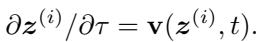
In the G-Adaptivity framework, this velocity is determined by a learnable diffusion process on the graph:

Here, \(\mathbf{A}_{\theta}\) is a learned “attention” matrix that describes how strongly connected nodes pull on each other.

How the Architecture Flows

Let’s visualize the entire process:

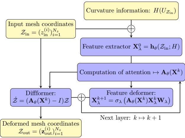
1. Input: We start with the current mesh coordinates and the curvature (Hessian) of the solution.
2. Attention: The network computes an attention matrix \(\mathbf{A}_{\theta}\). This determines the “weights” of the edges in the graph.
3. Diffusion: The mesh coordinates are updated by solving the diffusion equation (the “Diffformer” block).
4. Loop: This can be repeated in layers (blocks) to refine the movement.

3. Why It Doesn’t Tangle

Mesh tangling is the nightmare of r-adaptivity. Tangling happens when a node moves outside the element formed by its neighbors, causing triangles to overlap.

The Diffformer prevents this by design. Because the movement is based on graph diffusion, each node is effectively being pulled toward the weighted average of its neighbors.

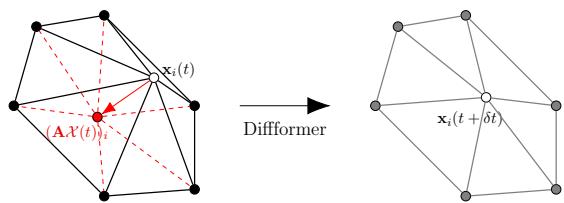
As shown in Figure 3, the diffusion process pulls a node \(\mathbf{x}_i\) into the convex hull (the geometric “safe zone”) of its neighbors.

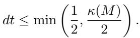
The authors provide a theorem proving that if the time-step of the diffusion is small enough (\(dt < 1/2\)), the mesh is mathematically guaranteed not to tangle.

4. Training with Direct Optimization

How does the network learn the optimal \(\mathbf{A}_{\theta}\)?

This is where the paper leverages modern differentiable programming. They use Firedrake, an automated FEM system. Because Firedrake can calculate gradients (derivatives) through the physics simulation itself (using the adjoint method), the system can calculate exactly how moving a mesh point \((x, y)\) affects the final error.

The loss function used for training has two parts:

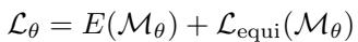
1. \(E(\mathcal{M}_{\theta})\): The actual Finite Element error (physics error).
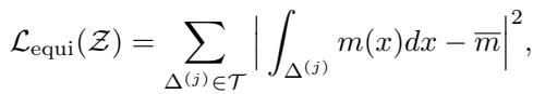
2. \(\mathcal{L}_{\mathrm{equi}}\): An “equidistribution” regularizer.

The regularizer helps stabilize training by encouraging the mesh to respect the “monitor function” concept from classical theory, even while the main objective minimizes the error directly.

Experiments and Results

The researchers tested G-Adaptivity on several standard physics problems.

1. Poisson’s Equation (Stationary)

Poisson’s equation is the “Hello World” of FEM. They tested it on a square domain and a complex polygonal domain.

Table 1 shows the results. G-Adapt achieves significantly higher error reduction (ER) than the classical Monge-Ampère (MA) method and the previous ML state-of-the-art (UM2N).

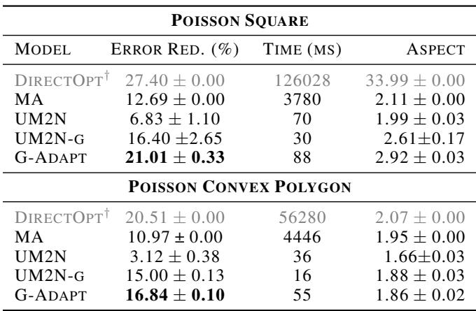
• Square Domain: G-Adapt reaches 21.01% Error Reduction (ER), beating MA (12.69%) and UM2N (6.83%).
• Speed: It runs in 88ms, compared to MA’s 3780ms.

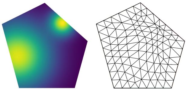
The method also works beautifully on irregular shapes. Below is the mesh generated for a polygonal domain. Notice how the triangles shrink (refine) around the areas of high solution intensity (the yellow spots on the left).

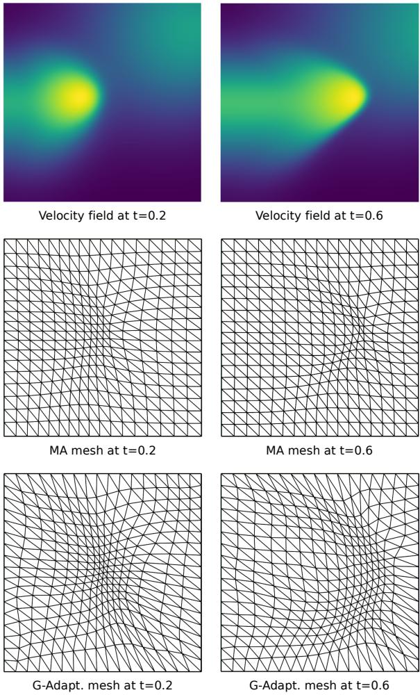
2. Burgers’ Equation (Time-Dependent)

Burgers’ equation involves a wave moving over time. This is harder because the mesh needs to evolve as the wave moves.

The authors tested a “rollout” scenario where they simulate 20 timesteps.

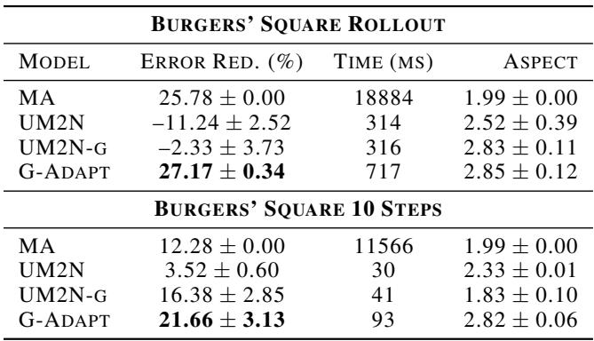
The results in Table 2 are striking. The previous ML baseline (UM2N) actually increased the error (negative reduction), likely because it couldn’t handle the shifting distribution of the wave. G-Adapt remained stable, achieving 27.17% error reduction, slightly beating the expensive classical MA method.

The visualization below shows the mesh tracking the velocity field over time.

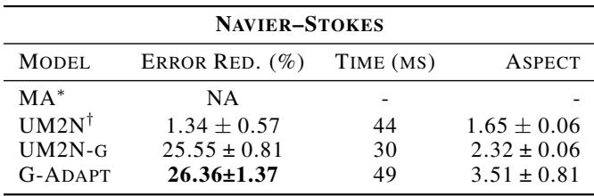
3. Navier-Stokes (Fluid Dynamics)

The final boss of these experiments is the Navier-Stokes equation, simulating flow past a cylinder. This involves complex interactions like vortex shedding (swirling flow behind the object).

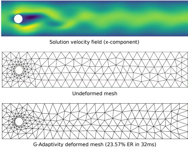
In Figure 6, you can see the mesh automatically refining:

1. At the “stagnation point” (front of the cylinder) where the fluid hits the object.
2. Along the “wake” behind the cylinder where vortices form.

Table 3 confirms that G-Adaptivity achieves 26.36% error reduction in just 49ms.

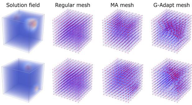
4. 3D and Scalability

Finally, the authors showed that the graph-based nature of their method allows it to scale easily to 3D and to much larger meshes than it was trained on (super-resolution).

Here is an example of a 3D cube mesh adapting to a central heat source.

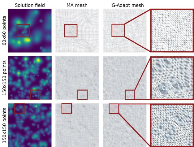
And here is the method scaling up to fine meshes (150x150) despite being trained on coarser ones.

Conclusion

The “G-Adaptivity” paper represents a significant step forward in scientific computing. By combining the geometric intuition of Graph Neural Networks with the rigorous math of Finite Element Methods, the authors have created a tool that is:

1. Fast: Orders of magnitude faster than solving Monge-Ampère equations.
2. Accurate: Directly minimizes physics error rather than just mimicking old heuristics.
3. Robust: Uses a diffusion-based architecture to mathematically guarantee the mesh doesn’t break.

This approach—using differentiable physics solvers to train neural networks to optimize simulation parameters—is likely the future of high-performance computing. It moves us away from purely data-driven “black boxes” toward “grey box” models that respect physical laws while exploiting the speed of AI.