Making LLMs Faster on the Edge: A Deep Dive into CHESS

The dream of running powerful Large Language Models (LLMs) like Llama-3 or Mistral directly on your laptop or phone—without relying on the cloud—is enticing. It promises privacy, lower latency, and offline capabilities. However, the reality is often a struggle against hardware limitations. These models are computationally heavy and memory-hungry.

One of the most effective ways to speed up these models is activation sparsification. The idea is simple: if a neuron’s activation value is close to zero, we can treat it as exactly zero and skip the math associated with it.

While this concept works beautifully for older models using ReLU activation functions (which naturally output lots of zeros), modern LLMs use sophisticated functions like SwiGLU. These functions improve intelligence but rarely output pure zeros, making sparsification difficult. Current methods try to force sparsity by cutting off small values, but they often do so blindly, hurting the model’s intelligence.

In this post, we will dive into a research paper that introduces CHESS (CHannel-wise thrEsholding and Selective Sparsification). The researchers propose a smarter, statistically grounded way to prune activations that speeds up inference by up to 1.27x with minimal accuracy loss.

The Problem: Why Simple Pruning Fails

To understand CHESS, we first need to look at the architecture of the Feed-Forward Networks (FFN) used in modern LLMs. The FFN module generally follows this structure:

Here, the input \(x\) is projected by a “gate” matrix and an “up” matrix. The gate is passed through an activation function \(\sigma\) (like SwiGLU), multiplied element-wise by the “up” projection, and finally projected “down.”

The intermediate activations are defined as:

The goal of sparsification is to set some elements of \(a^{\text{gate}}\) to zero so we can skip the subsequent multiplication operations. Existing methods, like a technique called CATS, use a simple threshold: if a value in \(a^{\text{gate}}\) is small, prune it.

The flaw in this approach is that it looks only at the magnitude of \(a^{\text{gate}}\). It ignores \(a^{\text{up}}\). However, if \(a^{\text{up}}\) is very large, even a small \(a^{\text{gate}}\) contributes significantly to the final output. Pruning it would cause a large error.

The CHESS Method

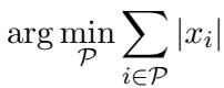
The authors of CHESS reformulate the problem. Instead of asking “Which values are small?”, they ask “Which values, if removed, will cause the least error in the next layer?”

1. Reformulating the Objective

The researchers mathematically define the objective as minimizing the difference between the original output and the sparsified output. We want to find a pruned version, \(\hat{a}^{\text{gate}}\), that solves this minimization problem:

By breaking this down, they derive a specific error calculation. To minimize the damage to the model, we should prune elements where the product of the “up” and “gate” activations is smallest. This leads to the definition of an importance score:

This equation reveals the core insight: you cannot decide to prune an activation based on the gate value alone; you must consider the “up” projection as well.

2. Channel-Wise Thresholding (CWT)

There is a computational catch. To calculate the exact importance score above, you have to compute \(a^{\text{up}}\) first. But the whole point of sparsification is to avoid doing extra computations. If we calculate everything just to decide what to delete, we haven’t saved any time.

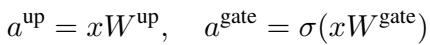
The researchers found a clever workaround by analyzing the statistical distribution of activations. They observed that while activation values vary wildly across different inputs, the average magnitude of \(a^{\text{up}}\) for a specific channel (column) remains consistent.

Take a look at the distributions below for three different channels in the Llama-3-8B model:

Notice how distinct the distributions are? Channel 1241 (left) centers around 3.5, while Channel 8718 (middle) clusters near 0. This stability allows the researchers to approximate the “up” value using its expected value (average) over a sample dataset:

By substituting this into the importance score, they create a new metric that doesn’t require computing \(a^{\text{up}}\) during inference. They then determine a specific threshold \(t_i\) for each channel \(i\). This is Channel-Wise Thresholding.

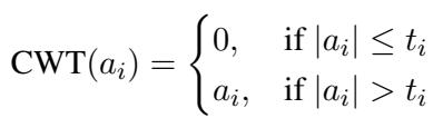
If an activation value is below its channel’s specific threshold, it gets zeroed out. This method respects the fact that some channels are naturally “louder” (have higher values) and require higher thresholds to be pruned effectively.

3. Selective Sparsification in Attention

While FFN layers consume the bulk of the parameters, the Attention modules also contribute to latency. However, Attention layers are sensitive. Pruning them aggressively usually breaks the model.

The authors applied a Taylor expansion analysis to the error function in attention projections.

Through simplification and analyzing the weights, they discovered that the rows in the weight matrices of attention projections have similar norms (magnitudes).

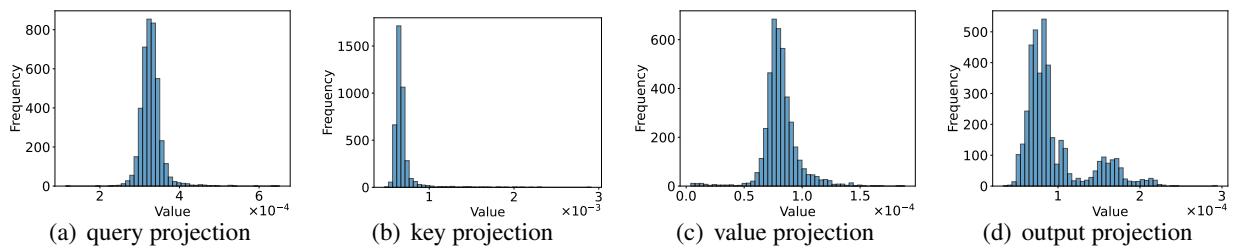
Because these norms are similar, the complex optimization problem simplifies back down to magnitude-based pruning for attention layers:

However, applying this to every part of the attention mechanism (Query, Key, Value, Output) causes too much accuracy loss. The researchers propose Selective Sparsification. They apply the thresholding only to the Query and Output projections, leaving the Key and Value projections untouched.

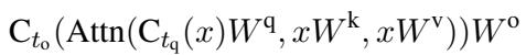
This strategy strikes a balance: it reduces memory access and computation enough to get speed gains, but preserves the critical information flow in the Key/Value pairs needed for accurate reasoning.

4. Efficient Sparse Kernels

Theoretical sparsity doesn’t automatically mean speed. Standard hardware (CPUs/GPUs) loves dense matrices. To realize the benefits of CHESS, the authors wrote custom software kernels.

They implemented two specific operations:

1. spvmm: Sparse Vector-Matrix Multiplication (used when the input vector is sparse).
2. vmmsp: Vector-Matrix Multiplication with Output Sparsity (used when we compute a dense vector but immediately mask it with zeros).

The performance difference is stark. The chart below compares the latency of the custom CHESS kernels (orange) versus standard PyTorch dense kernels (blue).

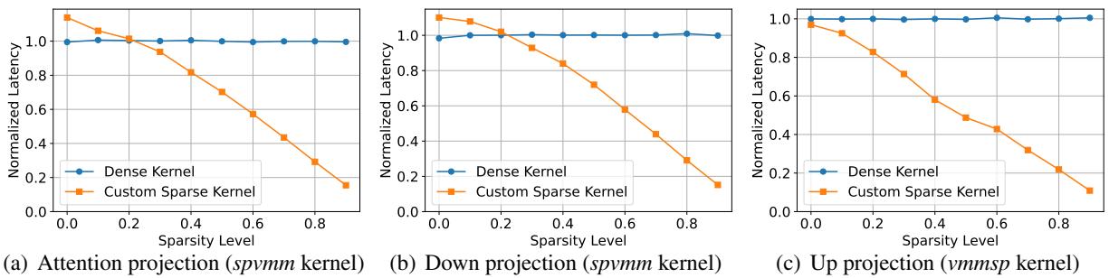
As the sparsity level (x-axis) increases, the custom kernels become significantly faster, whereas the standard kernels see almost no benefit.

Experimental Results

Does CHESS actually work? The researchers tested it on Llama-2 (7B, 13B, 70B), Llama-3-8B, and Mistral-7B across 8 standard downstream tasks (like ARC, HellaSwag, and PIQA).

Accuracy Retention

Table 1 below shows the results. CHESS w/ (with attention sparsification) and CHESS w/o (without) are compared against the Base model and the CATS method.

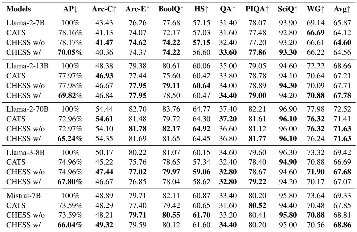
Key takeaways from the data:

• Lower Degradation: CHESS consistently outperforms CATS. For example, on Llama-3-8B, the average score for CHESS w/o is 67.68, significantly higher than CATS at 66.69.
• Robustness: Even when including attention sparsification (CHESS w/), the performance drop is minimal compared to the baseline, while CATS suffers more significant losses.

Speed Improvements

The primary goal was speed. The graph below illustrates the end-to-end inference speedup on a CPU.

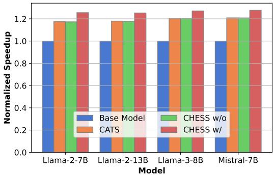
CHESS (the red bars) achieves the highest speedups across all models, reaching approximately 1.27x faster inference on Llama-3 and Mistral. This is a tangible improvement for real-time applications running on edge devices.

The Trade-off: Performance vs. Sparsity

Finally, it is important to visualize how the model behaves as we try to make it faster (more sparse).

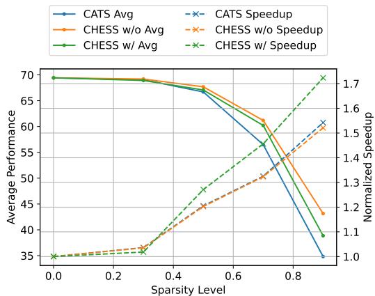
The green line (CHESS w/) shows the best trade-off. As sparsity increases (moving right on the x-axis), the speedup (dashed lines) rockets up. While accuracy (solid lines) inevitably drops at very high sparsity (>0.7), CHESS maintains usable performance much longer than CATS.

Conclusion

CHESS represents a significant step forward for deploying LLMs on consumer hardware. By moving away from simple magnitude-based pruning and reformulating the problem to account for the interactions between network layers, the researchers developed a method that is both faster and smarter.

The combination of Channel-Wise Thresholding (which respects the unique statistics of FFN channels) and Selective Sparsification (which carefully prunes specific parts of the Attention mechanism) allows LLMs to run more efficiently without needing expensive retraining. For students and developers looking to run Llama-3 on a laptop, CHESS offers a promising blueprint for the future of efficient AI.