Fast Forward: How to Speed Up LLM Finetuning by Just Keeping Going

Training Large Language Models (LLMs) is computationally expensive. Even as we’ve moved from training from scratch to fine-tuning pre-trained models, the cost in terms of time and GPU compute (FLOPs) remains a massive barrier for students and researchers.

To mitigate this, the community adopted Parameter Efficient Fine-Tuning (PEFT) methods, with LoRA (Low-Rank Adaptation) being the undisputed champion. LoRA reduces the memory footprint significantly by freezing the main model weights and training only a small subset of parameters. But here is the catch: while LoRA saves memory, it doesn’t necessarily speed up the training process itself by a huge margin. You still have to run thousands of iterations of Stochastic Gradient Descent (SGD).

But what if we could speed up the optimization process itself? What if standard optimizers like Adam are actually too cautious for the specific geometry of low-rank training?

In a fascinating paper titled “Fast Forwarding Low-Rank Training,” researchers propose a method that is almost suspiciously simple. They ask: If the optimizer tells us to move in a certain direction, why don’t we just keep moving in that direction until it stops helping?

This technique, called Fast Forward, results in up to an 87% reduction in FLOPs and an 81% reduction in training time, all without sacrificing model performance. In this post, we are going to tear down this paper, explain exactly how this algorithm works, and explore why “dumb” persistence might be the smartest way to train LoRA adapters.

The Problem with Modern Optimization

Before diving into the solution, we need to set the stage regarding how we currently train models. Modern machine learning relies heavily on optimizers like Adam or SGD (Stochastic Gradient Descent).

The standard loop looks like this:

1. Forward Pass: Pass data through the model to get a prediction.
2. Loss Calculation: Compare the prediction to the actual target.
3. Backward Pass (Backprop): Calculate gradients to see how each parameter contributed to the error.
4. Update: The optimizer nudges the weights slightly in the opposite direction of the error.

This process is repeated thousands of times. It is stable, but it is slow. Specifically, the Backward Pass is computationally expensive. Every single step requires calculating gradients for all trainable parameters.

The authors of this paper realized that in the specific context of Low-Rank training, the landscape of the loss function (the terrain we are trying to navigate to find the lowest point) is surprisingly smooth. If the terrain is smooth, taking tiny baby steps and checking your map (calculating gradients) every single second is inefficient. Sometimes, you just need to run down the hill.

Background: LoRA and the Low-Rank Landscape

To understand why Fast Forward works, we first need a quick refresher on LoRA.

When we fine-tune a massive model (like Llama-3 70B), updating every weight is impossible on consumer hardware. LoRA freezes the pre-trained weights (\(\mathbf{W}_0\)) and injects pairs of small trainable matrices (\(\mathbf{B}\) and \(\mathbf{A}\)) into the layers.

The update rule looks like this:

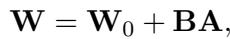
Here, \(r\) (the rank) is very small, often 8, 16, or 64. This forces the model to learn updates that exist in a “low-dimensional subspace.”

There is also a variation called DoRA (Weight-Decomposed Low-Rank Adaptation), which splits weights into magnitude and direction. The important takeaway for our purposes is that both methods constrain the movement of the model’s parameters. They don’t let the weights wander anywhere in the high-dimensional space; they are confined to a specific, lower-dimensional track.

It turns out that this constraint simplifies the geometry of the training. While full-rank training involves navigating a chaotic, bumpy landscape full of traps, low-rank training creates a smoother path. The researchers hypothesized that this smoothness could be exploited.

The Core Method: Fast Forward

The “Fast Forward” (FF) method is a hybrid optimization strategy. It alternates between two phases: the SGD Phase (standard training) and the Fast Forward Phase (acceleration).

The Algorithm

The concept is elegant in its simplicity. You start by training the model normally with Adam/SGD for a few steps to get a good sense of the direction. This is the “burn-in” or warmup. Once the optimizer has found a decent direction, you switch to Fast Forward.

Here is the visual breakdown of the algorithm:

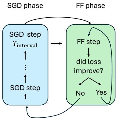
Let’s walk through the cycle shown in Figure 1:

1. SGD Phase: The model trains normally for a set number of steps (e.g., \(T_{interval} = 6\)). This allows the optimizer (Adam) to calculate momentum and determine a good update direction.
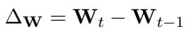
2. Calculate Direction (\(\Delta W\)): At the end of the SGD phase, we look at the difference between the current weights and the weights from the previous step. This vector represents the “velocity” and direction the optimizer wants to go.

3. Fast Forward Phase: Now, we stop doing backpropagation. We stop calculating gradients. Instead, we take the direction \(\Delta \mathbf{W}\) we just calculated and apply it repeatedly.

• Update 1: \(W_{new} = W + 1 \cdot \Delta W\)
• Update 2: \(W_{new} = W + 2 \cdot \Delta W\)
• Update 3: \(W_{new} = W + 3 \cdot \Delta W\)
• …and so on.

4. The Tiny Validation Set: How do we know when to stop? If we keep adding \(\Delta W\) forever, the model will eventually overshoot the valley and start climbing up the other side, increasing the loss. To prevent this, the authors use a tiny validation set (only about 32 examples). After every speculative jump in the Fast Forward phase, they check the loss on these 32 examples.

• Did loss improve? Yes \(\rightarrow\) Keep jumping.
• Did loss improve? No \(\rightarrow\) Stop! Revert to the last good step and go back to the SGD phase.

Why is this faster?

You might be wondering, “Wait, aren’t you still doing steps? How does this save time?”

The magic lies in the cost of the operations. In the Fast Forward phase, there is no backward pass. We are not calculating gradients. We are simply adding a matrix to the weights and running a forward pass to check loss.

A forward pass is significantly cheaper (roughly 3x faster) than a full training step (forward + backward + optimizer update). Furthermore, because the low-rank surface is smooth, the algorithm can often take many Fast Forward steps effectively skipping ahead in training without paying the expensive compute cost of backpropagation.

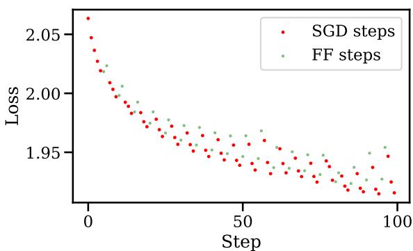
The visual impact on the training curve is striking. Look at the graph below:

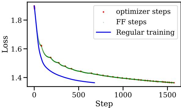
In Figure 4, the red dots are standard SGD steps. The green dots are Fast Forward steps. Notice how the loss drops vertically during the green sections? That is the algorithm “skiing” down the slope in a single direction, achieving in seconds what would normally take minutes of expensive compute. The blue line represents standard training—notice how Fast Forward achieves the same low loss much earlier.

Experiments and Results

The researchers validated this approach across several models (Pythia 1.4B to 6.9B, and Llama-3 8B) and distinct domains (Medical, Code Instruction, and Chat).

Massive Savings in FLOPs

The primary metric for efficiency in Deep Learning is FLOPs (Floating Point Operations). This measures the raw computational work done by the GPU.

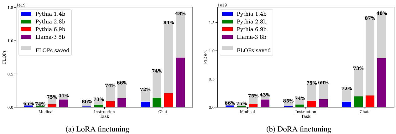
As shown in Figure 2, the results are consistent and dramatic.

• Medical Task: Saved up to 65-86% of FLOPs depending on the model size.
• Instruction Task: Saved 66-86%.
• Chat Task: Saved 48-84%.

The gray bars represent the work you don’t have to do. By simply repeating the last good step, the model reaches the target loss with a fraction of the calculation.

Savings in Wall-Clock Time

Theoretical FLOPs are nice, but does it actually save time on the clock? Yes.

Note: The image provided for Figure 3 in the deck seems to be Figure 14 in the description, or a mislabeled file. I will use images/004.jpg which corresponds to the time savings chart.

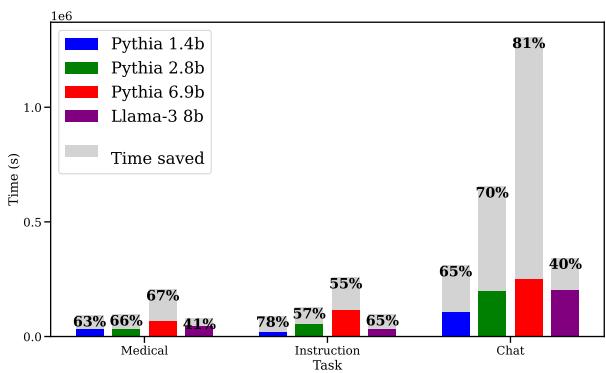
Figure 3 confirms that the FLOPs savings translate to real time. Training runs that usually take hours can be finished in roughly half the time. The savings are slightly lower than the FLOPs savings because running the validation check on the 32 examples does take some time, but the trade-off is overwhelmingly positive.

Does it hurt performance?

Speed is useless if the resulting model is stupid. The authors checked this rigorously.

1. Test Loss: The Fast Forward models converge to the same (or slightly better) loss values as standard training.
2. Benchmarks: They tested on PubMedQA. The standard model achieved 49.75% accuracy. The Fast Forward model achieved 50.95%.

Essentially, you get the same model, just faster.

Why Does It Work? (The Deep Dive)

This is the part that usually confuses students. We are taught that the loss landscape of a neural network is a non-convex nightmare of saddle points and local minima. Why on earth can we just walk in a straight line for 50 steps without crashing?

The answer lies in the Low-Rank constraint.

Convexity in Subspaces

The authors plotted the loss surface on a plane intersecting the pre-trained weights, the standard SGD weights, and the Fast Forward weights.

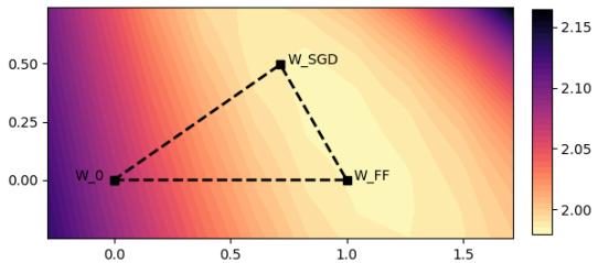
In Figure 5, look at how regular and “basin-like” the contours are. This suggests that in the specific subspace defined by LoRA, the loss function behaves very nicely. It is roughly convex.

Because the curve is convex (bowl-shaped), if you know the direction of the bottom of the bowl, you can take a big leap towards it. You don’t need to inch forward. This is conceptually similar to Line Search, a classic optimization technique from the pre-deep-learning era. Fast Forward is effectively performing a dynamic line search using the tiny validation set to determine the step size \(\tau\).

Gradient Consistency

Another fascinating finding involves how Fast Forward changes the training trajectory.

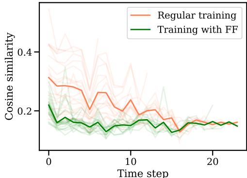
Figure 6 shows the cosine similarity between the current gradient and previous gradients.

• Orange Line (Regular): The gradients remain somewhat similar to previous steps.
• Green Line (Fast Forward): The similarity drops significantly.

This implies that when Fast Forward takes a big leap, it “exhausts” the potential of that specific direction. It squeezes all the juice out of that gradient. When the FF phase ends and SGD kicks back in, the optimizer is forced to find a new, different direction to improve the model. It stops the optimizer from redundantly retracing the same path step-by-step.

The Role of Rank

A counter-intuitive finding is related to the rank of the LoRA adapter. You might guess that as you increase the rank (adding more trainable parameters), the landscape would get more complex, and Fast Forward would fail.

The opposite happens.

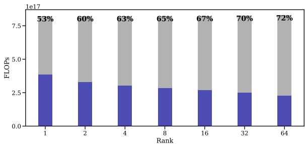
In Figure 7, we see that as the rank increases from 1 to 64, the savings (gray area) actually increase. Even at full rank (where \(r\) equals the model dimension), FF reduced FLOPs by 74% in one experiment.

This tells us that the success of Fast Forward isn’t just because the dimension is low; it’s likely due to the nature of the LoRA update matrices themselves.

When Does It Fail?

The authors were honest about limitations. They tried applying Fast Forward to Full-Rank Standard Fine-Tuning (updating all the weights of the model directly, no LoRA).

It failed completely.

As shown in Figure 8, the moment they tried to Fast Forward in full-rank training (green dots), the loss spiked immediately. Even a single speculative step was too much.

Why? The full-rank loss surface is not smooth. It is jagged. A direction that is good for step \(t\) is often terrible for step \(t+1\). The “Line Search” assumption holds for LoRA, but it breaks down for standard training. This suggests that LoRA acts as a regularizer that smooths the optimization landscape, enabling these aggressive speedups.

Optimizing the Fast Forward

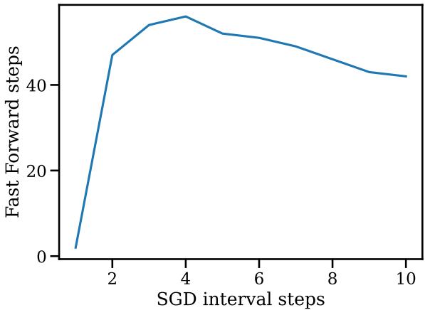
The paper also explores the hyperparameters of the method itself. For example, how long should you wait between Fast Forward bursts?

Figure 14 shows the relationship between the SGD interval (how many normal steps you take) and the Fast Forward length (how many cheap steps you get). It turns out you only need a very short SGD interval (about 4 steps) to get a massive run of Fast Forward steps (nearly 50!). If you wait too long (run SGD for 10 steps), the opportunity to “fast forward” actually decreases.

This suggests that the “direction” information in gradients expires quickly. You should calculate a direction, exploit it immediately with Fast Forward, and then recalculate.

Conclusion and Key Takeaways

The “Fast Forward” paper provides a refreshing perspective on training efficiency. While much of the industry focuses on hardware acceleration (better GPUs) or architectural changes (Mixture of Experts), this work highlights that we are leaving performance on the table simply because our optimizers are too conservative.

Here are the key takeaways for students and practitioners:

1. LoRA is Geometrically Unique: Low-Rank training creates a loss landscape that is much smoother than full-rank training.
2. Momentum is exploitable: If the optimizer points in a direction, you can likely follow that direction for a long time without recalculating gradients (in LoRA).
3. Forward vs. Backward: By trading expensive backward passes for cheap forward passes (on a tiny validation set), we can drastically cut compute costs.
4. Implementation: This method is relatively easy to implement on top of existing training loops. It requires no changes to the model architecture, only to the training loop logic.

As LLMs continue to grow, methods like Fast Forward that slash training costs by 80% without hardware upgrades will likely become standard tools in the machine learning engineer’s toolkit. Sometimes, the best way to get ahead is to stop overthinking and just keep moving forward.