](https://deep-paper.org/en/paper/2410.04074/images/cover.png)
If you have ever played with Word2Vec or early language models, you are likely familiar with the famous algebraic miracle of NLP: King - Man + Woman = Queen. This vector arithmetic suggested that language models (LMs) don’t just memorize text; they implicitly learn semantic and syntactic structures.
However, extracting that structure explicitly—drawing the actual grammar tree of a sentence—usually requires supervised training on expensive, hand-labeled datasets like the Penn Treebank. But what if we could get a pre-trained Large Language Model (LLM) to confess its grammatical knowledge without ever showing it a labeled parse tree?
In the paper “On Eliciting Syntax from Language Models via Hashing,” researchers from the National Institute of Information and Communications Technology (NICT) propose a fascinating method called Parserker2. By combining a classic dynamic programming algorithm (CKY) with modern contrastive learning and binary hashing, they manage to induce high-quality syntactic trees from raw text.
This post will walk you through how they upgraded the parsing mechanism from “zero-order” to “first-order,” how they turned parsing into a hashing problem, and the clever loss functions required to make unsupervised learning stable.
The Core Problem: Where is the Grammar?
Grammar is the invisible skeleton of language. In a sentence like “The quick brown fox jumps,” we know that “The quick brown fox” forms a Noun Phrase (NP) and “jumps” acts as the Verb (V). A Constituency Parser aims to recover this hierarchical tree structure.
Standard approaches usually follow a pipeline:
- Take a sentence.
- Encode it with a model (like BERT).
- Train a classifier on thousands of labeled trees to predict which words group together.
The researchers asked a harder question: Can we induce these trees using only the raw text and the pre-trained model’s internal knowledge?
To do this, they rely on a technique called Binary Representation. Instead of predicting a label like “NP” or “VP” from a fixed list, the model predicts a binary code (e.g., 10110...) for every span of text. If two spans act grammatically similar, they should have similar binary codes.
The Architecture at a Glance
Before diving into the math, let’s look at the high-level architecture.
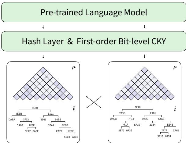
The model takes a sentence and passes it through a pre-trained LM (like BERT). It then uses a Hash Layer to produce scores, which are fed into a Bit-level CKY module. The output is a parse tree where every node is labeled with a hexadecimal hash code rather than a linguistic tag.
Background: The Limits of Zero-Order Parsing
To understand the innovation here, we need to revisit the CKY (Cocke-Kasami-Younger) algorithm. CKY is a bottom-up parsing algorithm used to find the most probable tree structure for a sentence. It works by combining smaller spans of text into larger ones.
In previous work (Parserker1), the authors used a Zero-order CKY. In this setup, the score of a span (a phrase like “the lazy dog”) depends only on the boundary tokens: the start (“the”) and the end (“dog”).
\[ g(l,r,c) = \dots \text{function of } h_l \text{ and } h_r \]While computationally efficient, this is linguistically weak. A phrase’s grammatical role isn’t determined just by its edges; it depends on its internal structure. Because zero-order parsing ignores the “split point” (where the phrase divides into children), it struggles to learn complex grammar in an unsupervised setting.
The Solution: First-Order Bit-Level CKY
The authors introduce First-order CKY. In this upgraded version, the score of a span depends on the splitting position (\(m\)).
Imagine parsing the phrase “The quick brown fox”.
- Zero-order asks: Do “The” and “fox” look like the edges of a valid phrase?
- First-order asks: If we split this at “brown” (The quick brown | fox), does the combination of the left child (“The quick brown”) and the right child (“fox”) make sense?
By incorporating the split point \(m\), the model unifies lexical information (the words) and syntactic information (how they combine) into a single representation.
Visualizing the Difference
The difference is best seen in the dynamic programming charts (grids used to calculate parse probabilities):
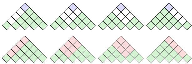
In the top triangle (Zero-order), the prediction relies on the top-most cell. In the bottom triangle (First-order), the prediction is a joint decision made by averaging cells crossing the left and right children.
The “Averaging” Trick
You might worry that checking every possible split point is too slow. If we have to compute complex neural network operations for every \(m\), the system becomes unusable.
The researchers found a clever mathematical shortcut. Instead of computing new vectors for every split, they simply average the scores of the constituent parts.
\[ \begin{array} { c } { \displaystyle { g ( l , r , m , c ) = \sum _ { k = 1 } ^ { K } g _ { k } ( l , r , m , c ^ { k } ) } } \\ { \displaystyle { g _ { k } ( l , r , m , + 1 ) = \frac { ( \mathbf { W } _ { k } ^ { Q } \overline { { h } } _ { l : m } ) ^ { \top } ( \mathbf { W } _ { k } ^ { K } \overline { { h } } _ { m + 1 : r } ) } { \sqrt { d _ { k } } } } } \\ { \displaystyle { \overline { { h } } _ { l : m } = \operatorname* { m e a n } _ { l \leq i \leq m } h _ { i } } } \\ { \displaystyle { \overline { { h } } _ { m + 1 : r } = \operatorname* { m e a n } _ { m < j \leq r } h _ { j } } } \end{array} \]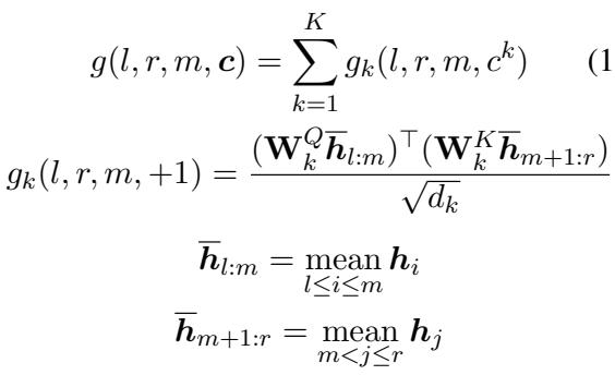
This equation essentially says: To get the representation of a span from \(l\) to \(m\), just take the mean of the hidden states in that range (\(\overline{h}_{l:m}\)). This allows the model to capture the “center of gravity” of a phrase, making the parsing sensitive to the internal structure without exploding computational cost.
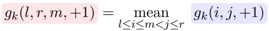
The calculation for a specific bit \(k\) being \(+1\) simplifies beautifully to averaging the scores of the sub-components:
Unsupervised Training via Contrastive Hashing
Now we have a mechanism (First-order CKY) to build trees. But how do we train it without labels? We don’t know if a span is an NP or a VP.
The answer is Contrastive Learning.
The intuition is simple: Identical phrases should have identical hash codes.
If the phrase “the lazy dog” appears in Sentence A and again in Sentence B, the model should assign them the same binary code (e.g., 1101), regardless of the context. Conversely, “the lazy dog” should have a different code from “jumps over”.
Defining Positives and Negatives
The model treats the parsing task as a self-supervised problem.
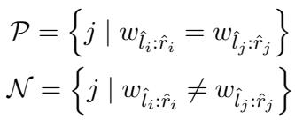
- Positive Set (\(\mathcal{P}\)): Spans that have the exact same text content (\(w_{\hat{l}_i:\hat{r}_i} = w_{\hat{l}_j:\hat{r}_j}\)).
- Negative Set (\(\mathcal{N}\)): Spans that have different text content.
Instead of maintaining a massive embedding table for every possible phrase (which would be millions of entries), the model uses Contrastive Hashing. It pulls the binary codes of positive pairs together and pushes negative pairs apart. This converts the “What label is this?” problem into a “Are these two the same?” problem, which is much easier to learn without supervision.
Generating the Binary Codes
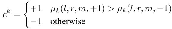
The binary code \(\mathbf{c}\) for a span isn’t arbitrary. It is derived from the marginal probabilities calculated by the CKY algorithm. If the probability of bit \(k\) being \(+1\) is higher than \(-1\), the code bit becomes \(+1\).
The Battle of Loss Functions
The most technical contribution of the paper—and the reason this method works where others failed—is the design of the loss function.
In standard contrastive learning (like SimCSE), you usually have one positive example and many negatives. But in parsing, a common phrase like “the” might appear dozens of times in a batch. You have multiple positives.
If you just take the average distance to all positives, the model gets confused (the “geometric center” issue). If you only look at the closest positive, the signal is too weak for a model with a large output space (like language).
The Proposed Solution: \(\ell_{\overline{\min}}\)
The researchers propose focusing on the hardest cases. They want to minimize the distance to the farthest positive instance (making the cluster tight) while maximizing the distance to the negatives.
However, simply using a min/max operator can destabilize training because the gradients get dominated by the positive terms. To fix this, they introduce a balanced loss function called \(\ell_{\overline{\min}}\).
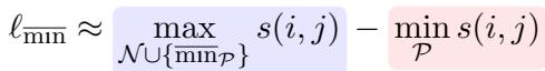
Here is the breakdown:
- \(\min_{\mathcal{P}}\) (The Pull): This term focuses on the “worst” positive match (the one furthest away) and tries to pull it closer. This provides a strong alignment signal.
- \(\overline{\min}_{\mathcal{P}}\) (The Balance): This term is added to the negative side. It is a “soft” version of the minimum operator (using LogSumExp). It ensures that the gradients from the positive term don’t overwhelm the gradients from the negative term.
This balance prevents the model from collapsing into trivial solutions (like right-branching trees) and forces it to learn meaningful structures.
Experiments and Results
Does it actually work? The researchers tested Parserker2 on the Penn Treebank (English) and the Chinese Treebank.
English Results (PTB)
On the Penn Treebank, the model achieves competitive F1 scores compared to other unsupervised methods.
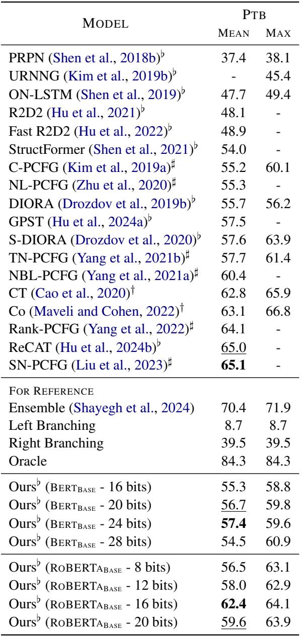
As shown in Table 1, “Ours” (Parserker2) consistently outperforms implicit grammar models (like ON-LSTM and PRPN). It achieves an F1 score of 57.4 with 24 bits using BERT-Base, which is impressive given it uses no labeled data.
Chinese Results (CTB)
The results on Chinese are even more striking. Chinese syntax is notoriously difficult for unsupervised models.
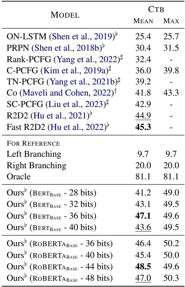
Table 2 shows that Parserker2 outperforms almost all baselines by a significant margin. Interestingly, the model required more bits (36-44 bits) to reach peak performance on Chinese compared to English, suggesting that capturing Chinese syntax requires a higher-dimensional binary space.
Seeing the Matrix: What do the trees look like?
The numbers are good, but the visualizations are better. Since the model outputs trees with hexadecimal labels, we can compare them to ground-truth trees.
Take the sentence: “The quick brown fox jumps over the lazy dog.”
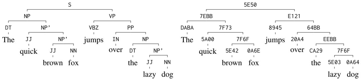
In the image above:
- Left: The human-annotated tree with tags like NP (Noun Phrase) and VP (Verb Phrase).
- Right: The model’s output with hex codes.
Notice that the structure is identical.
- The model correctly groups “The quick brown fox” under one node (
7EBB). - It groups “the lazy dog” under another node (
EEBB). - Crucially, the codes for similar concepts are similar. Preterminal adjectives like “quick” (
5A00) and “brown” (5E42) share bits, showing the model has learned parts of speech.
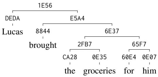
Handling Complexity
The model scales well to longer, more complex sentences. Below is a deeper tree derivation. Notice how the hierarchy is preserved all the way from the root node down to individual tokens.
Conclusion
The “Parserker2” paper demonstrates a significant leap in unsupervised syntax induction. By moving from zero-order to first-order CKY, the researchers enabled the model to consider the internal structure of spans, not just their boundaries. By employing contrastive hashing with a carefully balanced loss function, they managed to train this complex structure using nothing but raw text.
This work implies that high-quality syntactic annotations—usually a bottleneck in NLP—can be acquired at a very low cost. The binary codes generated by the model are not just random numbers; they are a compressed, discrete representation of the “grammar” that LLMs have been hiding from us all along.
For students and researchers, this is a powerful reminder: sometimes the best way to understand a neural network is not to add more layers, but to impose the right structural constraints (like CKY) and ask the right questions (like “are these two spans identical?”).