Introduction

In the current landscape of Artificial Intelligence, Large Language Models (LLMs) like GPT-4, PaLM, and LLaMA have become the cornerstones of Natural Language Processing. They possess incredible capabilities, but they come with a hefty price tag: inference efficiency. Running these massive models—often containing billions of parameters—is resource-intensive. For companies offering “Language Model as a Service,” handling concurrent queries from thousands of users creates a massive bottleneck.

Imagine a bus (the GPU) that is designed to carry only one passenger (a user query) at a time. To transport 30 people, the bus has to make 30 separate trips. This is essentially how standard serial inference works. It is slow and computationally expensive.

To solve this, researchers have been exploring Data Multiplexing. This is the equivalent of figuring out how to seat multiple passengers on that single bus trip. By merging multiple inputs into a single composite representation, we can run the heavy computational “forward pass” of the LLM just once for several users.

However, there is a catch. When you mix different queries together, the model often gets confused. It struggles to distinguish which output belongs to which input, leading to “hallucinated” or mixed-up answers. Previous solutions required retraining the entire LLM to understand this mixing process—a task that is practically impossible with today’s massive, pre-trained models.

Enter RevMUX. In a recent paper, researchers introduced a parameter-efficient framework that allows us to mix inputs (multiplexing) and separate outputs (demultiplexing) without ever needing to retrain the massive backbone model. The secret sauce? Reversible Adapters.

In this post, we will tear down the RevMUX architecture, explain the mathematics behind its reversible design, and look at how it manages to speed up inference while keeping accuracy high.

Background: The Inference Bottleneck

Before diving into RevMUX, we need to understand the landscape of efficient inference. The community generally tackles the slowness of LLMs in two ways:

1. Model-Centric Approaches: These methods try to make the model itself smaller or simpler. Techniques like Quantization (turning high-precision 32-bit weights into 8-bit or 4-bit) and Pruning (removing redundant connections) fit here. While effective, they physically alter the model.
2. Algorithm-Centric Approaches: These optimize how the calculation is done, such as Speculative Decoding or optimizing the Key-Value (KV) Cache.

However, neither of these solves the specific problem of batch throughput without increasing the computational load linearly. If you have 10 inputs, you usually do 10x the work.

Multi-Input Multi-Output (MIMO)

The concept of Multi-Input Multi-Output (MIMO) learning proposes a radical shift: process multiple inputs in a single pass.

In a standard MIMO setup (specifically DataMUX), a “Multiplexer” layer combines inputs \(x_1\) and \(x_2\) into a single vector. The neural network processes this vector. Then, a “Demultiplexer” layer tries to tease apart the results into \(y_1\) and \(y_2\).

The problem with previous attempts at this, like MUX-PLMs, is that they require end-to-end training. You have to update the weights of the BERT or GPT model so it “learns” how to handle these mixed signals. For an 8-billion or 70-billion parameter model, fine-tuning the whole thing just for inference speed is costly and creates storage nightmares (you’d need a different copy of the model for every different compression rate).

This is where RevMUX changes the game. It asks: Can we create a smart adapter that mixes and unmixes data so perfectly that the LLM doesn’t even know it’s processing multiple inputs at once?

The Core Method: RevMUX

RevMUX (Reversible Multiplexing) is designed to work with a fixed, frozen backbone LLM. It wraps the model in a sandwich of adapters: a Multiplexing Layer at the start and a Demultiplexing Layer at the end.

Let’s look at the high-level comparison between traditional processing, DataMUX, and the new RevMUX architecture.

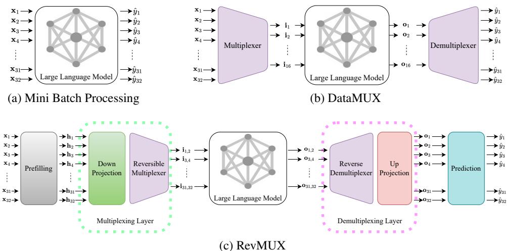
As seen in Figure 1:

• (a) Mini Batch: Every input (\(x_1\) to \(x_{32}\)) gets its own lane. Accurate, but slow.
• (b) DataMUX: Squeezes inputs together, but relies on the model being trained to handle the squeeze.
• (c) RevMUX: Uses a specific “Reversible Multiplexing” layer. It takes inputs, projects them down, mixes them reversibly, passes them through the frozen LLM, and then unmixes them.

Let’s break down the three distinct stages of the RevMUX pipeline.

1. Prefilling: Aligning the Feature Space

When you mash two sentences together mathematically, the resulting vector often looks nothing like a real sentence. This is called a distribution shift. If you feed this “weird” vector into a frozen LLM, the model won’t know what to do with it because it hasn’t seen data like this during pre-training.

To fix this, RevMUX uses a Prefilling step. Before mixing, the inputs are processed by the first few layers of the LLM (or a prompt encoder) to convert raw text into a dense representation that the model “likes.”

\[ \mathbf { h } _ { k } ^ { l } = \operatorname { E n c o d e r } _ { 0 : l } ( \mathbf { X } _ { k } ) , \]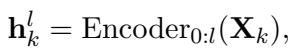

Here, the inputs are passed through the first \(l\) layers of the encoder. This ensures the features are in the correct semantic space before we start mixing them.

2. The Multiplexing Layer

This is the heart of the innovation. The goal is to combine \(N\) inputs into one. For this explanation, let’s assume we are mixing 2 inputs (\(N=2\)).

First, the high-dimensional vectors are projected down to save space:

\[ \mathbf { i } _ { k } ^ { l } = f _ { \mathrm { d o w n } } ( \mathbf { h } _ { k } ^ { l } ) . \]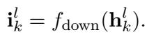

Next comes the Reversible Multiplexer. Inspired by Reversible Neural Networks (RevNets), this module splits the inputs and mixes them in a way that is mathematically guaranteed to be separable.

Unlike a simple addition (\(A + B = C\), where you can’t get A back if you only know C), RevMUX uses a system of coupled functions.

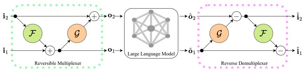
As shown in Figure 2 (left side), the mixing happens in two stages using learnable functions \(\mathcal{F}\) and \(\mathcal{G}\) (which are small Multi-Layer Perceptrons).

The equations for mixing are:

\[ \begin{array} { r l } & { \mathbf { o } _ { 1 } ^ { l } = \mathbf { i } _ { 1 } ^ { l } + \mathcal { F } ( \mathbf { i } _ { 2 } ^ { l } ) , } \\ & { \mathbf { o } _ { 2 } ^ { l } = \mathbf { i } _ { 2 } ^ { l } + \mathcal { G } ( \mathbf { o } _ { 1 } ^ { l } ) , } \\ & { \mathbf { o } ^ { l } = \mathrm { c o n c a t } [ \mathbf { o } _ { 1 } ^ { l } , \mathbf { o } _ { 2 } ^ { l } ] , } \end{array} \]

Notice the dependency chain:

1. Output 1 (\(o_1\)) is Input 1 plus a transformation of Input 2.
2. Output 2 (\(o_2\)) is Input 2 plus a transformation of the already calculated Output 1.

This combined output \(o^l\) is then sent through the massive, frozen LLM.

\[ \hat { \mathbf { o } } = \mathrm { D e c o d e r } \Big ( \mathrm { E n c o d e r } _ { l + 1 : L } \big ( \mathbf { o } ^ { l } \big ) \Big ) , \]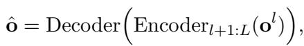

The LLM does its heavy lifting here. Because inputs are combined, the LLM only runs once, saving significant computational resources (FLOPs).

3. The Demultiplexing Layer

After the LLM produces the output, we have a mixed result vector. We need to disentangle it to get the specific predictions for User 1 and User 2.

Because the multiplexer was designed reversibly, the demultiplexer is simply the mathematical inverse. We don’t need to “guess” how to separate them; we calculate it.

Looking at Figure 2 (right side) and the equations below, we reverse the operations in the exact opposite order:

\[ \begin{array} { r } { \left[ \hat { \bf 0 } _ { 1 } , \hat { \bf 0 } _ { 2 } \right] = \hat { \bf 0 } , \qquad } \\ { \hat { \bf i } _ { 2 } = \hat { \bf 0 } _ { 2 } - \mathcal { G } ( \hat { \bf 0 } _ { 1 } ) , \qquad } \\ { \hat { \bf i } _ { 1 } = \hat { \bf 0 } _ { 1 } - \mathcal { F } ( \hat { \bf i } _ { 2 } ) , \qquad } \end{array} \]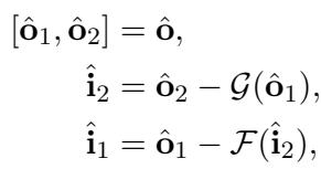

1. First, we recover Input 2 by subtracting the transformation of Output 1.
2. Then, having recovered Input 2, we use it to recover Input 1.

Finally, we up-project the vectors back to the original dimension (\(f_{up}\)) and generate the classification label using the prediction head.

\[ \begin{array} { r } { \hat { \bf h } _ { k } = f _ { \mathrm { u p } } ( \hat { \bf i } _ { k } ) , } \end{array} \]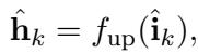

Training RevMUX: The Loss Functions

The beauty of this system is that we only train the small adapters (\(\mathcal{F}\), \(\mathcal{G}\), \(f_{down}\), \(f_{up}\)). The billions of parameters in the LLM stay untouched.

To train these adapters, the authors use two loss functions combined:

1. Cross-Entropy Loss (\(\mathcal{L}_{ce}\)): This is the standard “did we get the right answer?” loss. It compares the model’s prediction to the true label (Gold Label).

2. InfoNCE Loss (\(\mathcal{L}_{info}\)): This is crucial. Since the backbone LLM is frozen, it expects inputs that look a certain way. If our demultiplexed output looks like garbage, the final classification head will fail. InfoNCE is a contrastive loss. It forces the representation coming out of the Demultiplexer (\(\hat{h}_k\)) to be as similar as possible to the representation the model would have produced if we ran the input normally (one-by-one).

   \[ \begin{array} { l } { { \displaystyle { \mathcal L } _ { \mathrm { i n f o } } = \sum _ { k = 1 } ^ { N } \mathrm { I n f o N C E } ( \hat { \bf h } _ { k } , { \bf h } _ { k } ) } , \ ~ } \\ { { \displaystyle = \sum _ { k = 1 } ^ { N } - \mathbb E [ \log \frac { \exp ( \hat { \bf h } _ { k } \cdot { \bf h } _ { k } ) } { \exp ( \hat { \bf h } _ { k } \cdot { \bf h } _ { k } ) + \sum _ { j \ne k } ^ { N } \exp ( \hat { \bf h } _ { k } \cdot { \bf h } _ { j } ) } ] } } \end{array} \]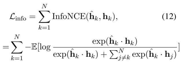

   

This loss function essentially tells the adapters: “Make sure the recovered vector for User 1 looks exactly like User 1’s original vector, and distinct from User 2’s vector.”

Experimental Results

The theory sounds solid, but does it work? The researchers tested RevMUX on three different LLM architectures: BERT (Encoder-only), T5 (Encoder-Decoder), and LLaMA-3 (Decoder-only), using datasets from the GLUE benchmark (like SST-2 for sentiment analysis).

1. Performance vs. Baselines

The first major test was on BERT-Base. They compared RevMUX against:

• DataMUX: The previous state-of-the-art that trains the whole model.
• MUX-PLM: Another full-training method.
• Vanilla Adapters: A simplified version of RevMUX without the “reversible” math.

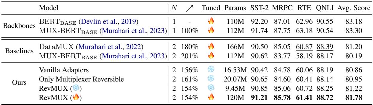
Table 1 reveals several key findings:

• RevMUX (❄️ Frozen) achieves performance comparable to fully fine-tuned baselines. This is remarkable because RevMUX only updates a tiny fraction of the parameters compared to DataMUX.
• Reversibility Matters: RevMUX consistently outperforms “Vanilla Adapters.” This proves that the specialized reversible architecture is doing the heavy lifting in preserving signal integrity during the mixing process.
• Speedup: With \(N=2\) (mixing 2 inputs), the model achieves roughly a 1.5x to 1.6x speedup in inference compared to processing inputs one by one.

2. The Efficiency-Accuracy Trade-off

There is always a price to pay for speed. In data multiplexing, the price is usually a drop in accuracy.

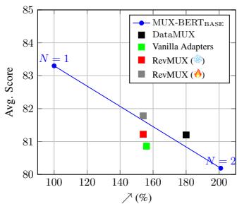
Figure 3 illustrates this trade-off.

• The x-axis represents efficiency (throughput), and the y-axis is accuracy.
• The blue line represents the ideal baseline.
• The Red Circle (RevMUX) sits higher than the Black Square (DataMUX) for the same efficiency.

This visualizes that for every unit of speed gained, RevMUX sacrifices less accuracy than its competitors. It effectively “bends the curve” of the trade-off.

3. Scalability to Larger Models (T5)

Does this only work on small models like BERT? The authors tested it on T5 at three different scales (Small, Base, Large).

Table 2 shows that RevMUX scales well. On T5-Large, running with \(N=2\) provided a 143% speedup while keeping the average score very close to the baseline.

• T5-Large Baseline (N=1): 91.93 Avg Score
• RevMUX (N=2): 82.64 Avg Score

While there is a drop in performance (which is expected when compressing 2 inputs into 1), the speed gain is massive. Note that larger models (\(T5_{Large}\)) showed slightly more degradation than smaller ones, highlighting a challenge in scaling this to massive dimensions.

4. What is the impact of Batch Size (\(N\))?

How many inputs can we squeeze together? 2? 4? 16?

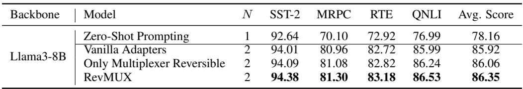
Figure 4 plots accuracy against the number of mixed samples (\(N\)).

• As \(N\) increases (moving right on the x-axis), accuracy naturally drops. The model has to “remember” too many distinct inputs in a single vector.
• The Role of Prefilling (\(l\)): The different colored lines represent different amounts of “Prefilling” layers. Notice that \(l=6\) (Green line) often sustains higher accuracy at larger \(N\) compared to \(l=0\) (Blue dashed line). This confirms that preprocessing the features before mixing them is critical for high-load multiplexing.

5. Does the InfoNCE Loss Help?

Finally, an ablation study was conducted to see if that complex contrastive loss function (\(\mathcal{L}_{info}\)) was actually necessary.

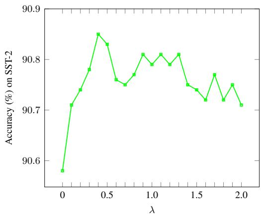
Figure 6 shows the accuracy on SST-2 as the weight of the InfoNCE loss (\(\lambda\)) changes.

• When \(\lambda = 0\) (no InfoNCE), accuracy is lower (~90.6%).
• As \(\lambda\) increases to around 0.5 - 1.0, accuracy peaks (~90.9%).
• This confirms that forcing the demultiplexed vectors to resemble the original vectors helps the frozen backbone model make better predictions.

Conclusion and Implications

RevMUX represents a significant step forward in “Green AI” and efficient computing. By leveraging the mathematical properties of reversible neural networks, the authors have created a way to “cheat” the system—processing multiple inputs for the price of one, without having to retrain the expensive backbone model.

Key Takeaways:

1. Plug-and-Play: RevMUX works on frozen models, making it applicable to today’s massive LLMs where retraining is impossible for most users.
2. Reversibility is Key: The reversible adapter design allows for better signal reconstruction than standard linear layers used in previous methods.
3. Flexible Efficiency: Users can choose their trade-off. If they need 100% accuracy, they use standard inference. If they need 2x speed and can tolerate a 2-5% drop in accuracy, they can switch on RevMUX with \(N=2\).

As LLMs continue to grow in size, techniques like RevMUX that optimize the “serving” side of the equation will become just as important as the models themselves. It opens the door for real-time applications on edge devices and lowers the carbon footprint of large-scale AI services.

---