](https://deep-paper.org/en/paper/2410.05331/images/cover.png)
The release of Large Language Models (LLMs) currently faces a massive dilemma. On one hand, you have the “walled garden” approach (like OpenAI’s GPT-4 or Anthropic’s Claude), where models are hidden behind APIs. This protects the developers’ intellectual property but forces users to send their private data to third-party servers, raising massive privacy concerns.
On the other hand, you have the open-source approach (like Llama or Mistral), where weights are released publicly. This is great for user privacy—you can run the model locally—but it’s a nightmare for developers who lose ownership and control over their models. Once the weights are out, bad actors can use them for unethical purposes or competitors can use them for commercial gain without permission.
Is there a middle ground? Can we release a model that runs locally (protecting user privacy) but keeps the actual weights secret (protecting developer ownership)?
Researchers from Rice University and collaborators have proposed a fascinating solution named TaylorMLP. By leveraging the mathematical power of Taylor Series expansions, they have found a way to “encrypt” model weights into a new format. This allows users to run the model locally but—crucially—makes the generation process slower, preventing large-scale commercial abuse. They cheekily dub this slowing mechanism “Taylor Unswift.”
In this post, we’ll break down exactly how TaylorMLP works, the math behind the weight transformation, and why this might be the future of secure model distribution.
The Access Dilemma
To understand why TaylorMLP is necessary, we first need to visualize the current landscape of LLM distribution.
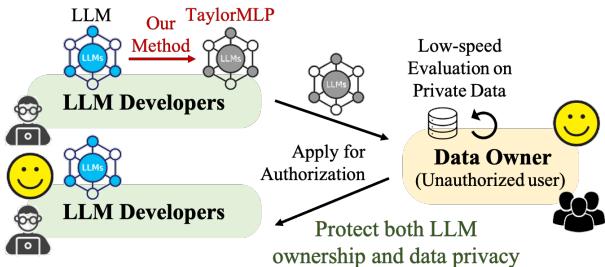
As shown in Figure 1:
- API Release (a): The developer keeps the model safe, but the user must upload private data.
- Open Source (b): The user keeps their data safe, but the developer loses ownership of the model.
- TaylorMLP (c): The goal is to allow users to evaluate the model on private data without the developer giving away the raw model weights.
The core idea is to transform the model into a format that is mathematically equivalent in output but structurally different in a way that hides the original parameters.
Background: The MLP Layer
To protect an LLM, we need to look at its building blocks. Transformer models (the architecture behind almost all modern LLMs) consist of Attention layers and Multi-Layer Perceptron (MLP) layers.
A standard MLP layer usually follows this pipeline:
- Linear Projection: Input \(x\) is multiplied by weights.
- Activation: A non-linear function (like GELU or SiLU) is applied.
- Linear Projection: The result is multiplied by another set of weights.
Mathematically, the output \(y_i\) of a specific dimension in an MLP layer looks like this:
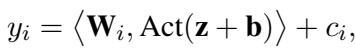
Here, \(\mathbf{W}\) and \(\mathbf{b}\) are the weights and biases we want to protect. If you give these to the user, you’ve given away the model. TaylorMLP proposes a method to replace these specific matrices with a different set of parameters derived from Calculus.
The Core Method: Taylor Expansion
If you remember your undergraduate calculus, a Taylor Series allows you to approximate a complex function as an infinite sum of terms calculated from the values of its derivatives at a single point.
The researchers realized that the activation functions in LLMs (like GELU) can be expanded using a Taylor series. By doing this, they can mix the weight matrices into the polynomial coefficients.
1. The Architecture Shift
Let’s compare the standard architecture with the TaylorMLP architecture.
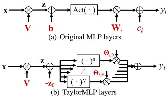
In Figure 2(a), you see the standard path: \(x \to z \to \text{Act}(z+b) \to y\). In Figure 2(b), the explicit weights \(\mathbf{b}\), \(\mathbf{W}\), and \(\mathbf{c}\) are gone. Instead, we have a series of parallel branches representing different orders of the Taylor expansion (\(N=0\) to \(N\)).
2. The Math Behind the Magic
How do we get rid of the weights? We start by expanding the activation term \(\text{Act}(\mathbf{z} + \mathbf{b})\) around a “local embedding” point \(\mathbf{z}_0\).
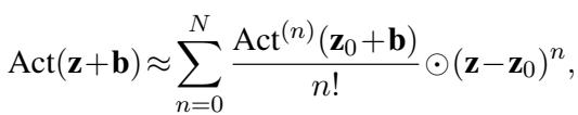
This equation looks complex, but it’s just a standard Taylor expansion. The interesting part happens when we substitute this expansion back into the original MLP equation. By rearranging the terms, the researchers merge the original weights \(\mathbf{W}\) with the derivatives of the activation function.
This leads to the definition of the Latent Parameters, denoted as \(\Theta\) (Theta).
The crucial innovation here is Equation (3) above. The output \(y_i\) is now calculated using \(\Theta_{i,n}\) and the input data. The original weights \(\mathbf{W}\) and biases \(\mathbf{b}\) are “baked into” these \(\Theta\) parameters.
The definitions of these new safe parameters are:
Why is this secure? You (the user) are given \(\Theta\). To get back the original \(\mathbf{W}\) and \(\mathbf{b}\), you would need to reverse-engineer the Taylor series combination. The paper demonstrates that this process is effectively irreversible because multiple combinations of weights could potentially produce similar \(\Theta\) values, and without the original seeds, reconstruction is infeasible.
3. The “Unswift” Mechanism (Slowing Down Generation)
You might wonder, “If the output is the same, why does this prevent abuse?”
The answer lies in Computational Complexity. In a standard MLP, you do one pass. In TaylorMLP, to get an accurate result, you must sum up multiple terms of the series (from \(n=0\) to \(N\)).
- If \(N=0\), the model is fast but inaccurate (hallucinates).
- If \(N=8\), the model is accurate but requires many more Floating Point Operations (FLOPs).
The researchers call this intentional delay “Taylor Unswift.” It increases the latency by roughly \(4\times\) to \(10\times\).
This is a feature, not a bug. It allows individual researchers or developers to test the model on their private data (where speed isn’t critical), but it makes it economically unviable for a competitor to take this model and serve it to millions of users via a commercial API.
4. Convergence
Does this approximation actually work? Theoretically, yes. As the number of terms (\(N\)) approaches infinity, the TaylorMLP output becomes identical to the original MLP output.
However, we can’t calculate infinite terms. We need to find a “sweet spot” for \(N\) where the model is accurate enough to be useful but slow enough to be protected.
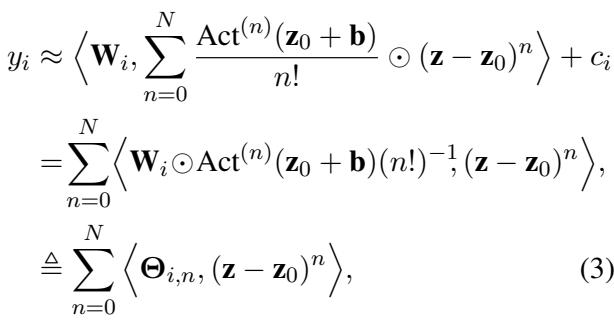
5. Derivatives of Activation Functions
To make this work, we need high-order derivatives of functions like GELU and SiLU. These get complicated quickly. The visualizations below show how the derivatives of GELU behave as the order (\(n\)) increases.
As \(n\) increases (going from a to f), the function becomes increasingly oscillatory. The TaylorMLP method relies on accurately computing these shapes to reconstruct the activation behavior.
Experimental Results
The researchers tested TaylorMLP on three major model families: Llama-3-8B, Mistral-7B, and Phi-2. They evaluated both the accuracy preservation and the latency increase.
RQ1: Accuracy vs. Latency
The most critical question is: Does the model still work?
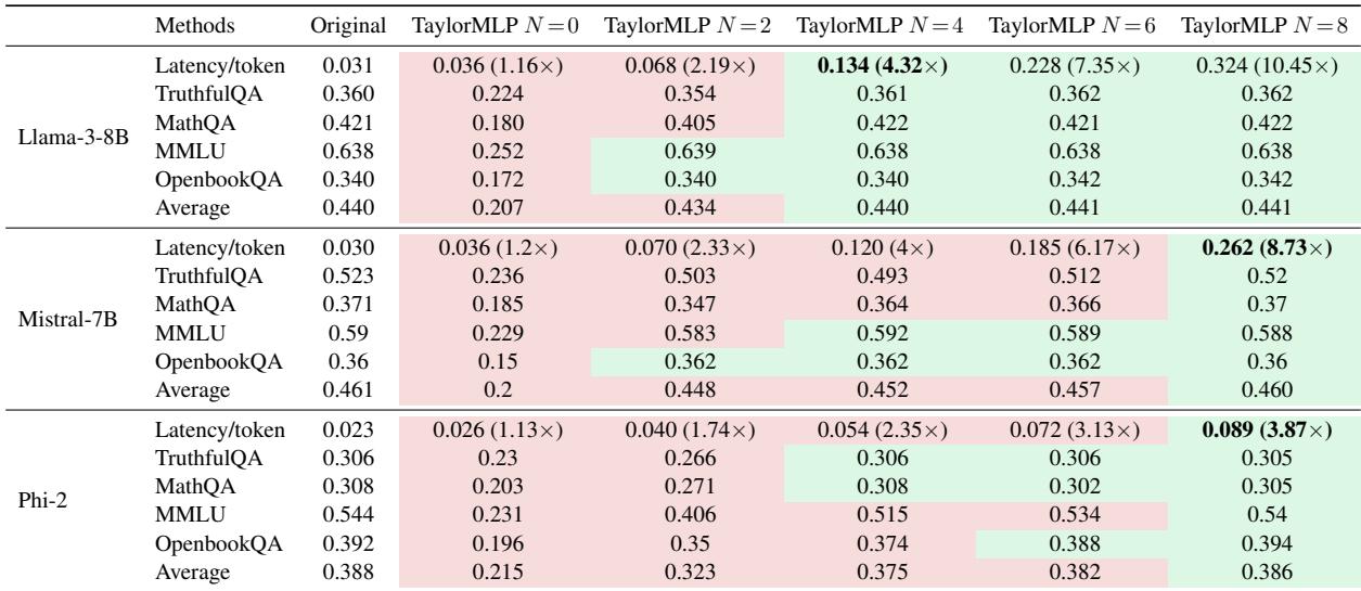
Key Takeaways from Table 1:
- Accuracy Recovery: Look at the columns for \(N=0\) vs \(N=8\). At \(N=0\), the accuracy (e.g., on MMLU) drops significantly. However, at \(N=8\), the accuracy is almost identical to the “Original” column.
- Latency Increase: Now look at the “Latency/token” rows. For Llama-3-8B, the original latency is 0.031s. At \(N=8\), it jumps to 0.324s—a 10.45x increase.
This confirms the “Unswift” hypothesis: the model becomes accurate but significantly slower.
RQ2: Can the Weights be Stolen?
The researchers simulated attacks where “unauthorized users” tried to reconstruct the model using fine-tuning and distillation.
Fine-Tuning Attack: Attackers tried to re-initialize the weights and fine-tune the model on downstream datasets (TruthfulQA, MathQA, etc.) to see if they could recover performance.
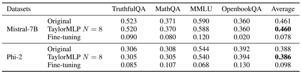
As shown in Table 2, the fine-tuned models (simulating stolen weights) performed terribly (e.g., 0.120 on MMLU vs 0.588 for TaylorMLP). This proves that simply having the architecture and datasets isn’t enough; you need the specific protected weights.
Distillation Attack: Attackers tried to “distill” the knowledge from the TaylorMLP model into a standard, fast model.
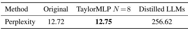
Table 3 shows that the distilled model had a perplexity of 256.62 (lower is better), compared to 12.75 for TaylorMLP. The distilled model was essentially garbage, producing hallucinations.
RQ3: How Many Terms (\(N\)) Do We Need?
The relationship between the expansion order \(N\) and performance is visualized clearly in Figure 5.
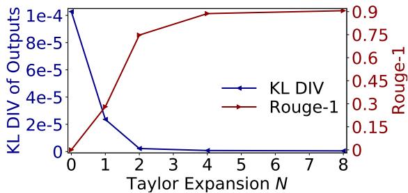
- Blue Line (KL Divergence): This measures how different the output probability is from the original model. It drops to near zero around \(N=4\) to \(N=8\).
- Red Line (ROUGE-1): This measures text overlap. It climbs back to nearly 1.0 (perfect match) as \(N\) increases.
This suggests that \(N=8\) is the magic number for maintaining quality.
Conclusion and Implications
TaylorMLP represents a novel approach to the “Open Weight” vs. “API” debate. It creates a new category of model release: Secured Weights.
Why does this matter?
- Try Before You Buy: Users can download a TaylorMLP version of a proprietary model. They can run it on their sensitive medical or financial data to see if it works without leaking data to the developer.
- Intellectual Property Protection: Developers can release these “demo” versions without fear that a competitor will spin up a high-speed API service using their hard work, thanks to the latency penalty.
- Regulatory Compliance: This allows for secure auditing of models in restricted environments.
By transforming weights into Taylor-series parameters, TaylorMLP ensures that the “secret sauce” of the model remains hidden, while the functional utility—albeit in “slow motion”—remains accessible to the world. It’s a clever application of fundamental calculus to solve a very modern AI problem.