](https://deep-paper.org/en/paper/2410.08027/images/cover.png)
Keeping Secrets in High Dimensions: A New Approach to Private Word Embeddings
Natural Language Processing (NLP) has become deeply embedded in our daily lives, from the predictive text on your smartphone to the large language models (LLMs) analyzing medical records. However, these models have a tendency to be a bit too good at remembering things. They often memorize specific details from their training data, which leads to a critical problem: privacy leakage. If a model is trained on sensitive emails or clinical notes, there is a risk that an attacker could extract that private information.
To combat this, researchers turn to Differential Privacy (DP)—a mathematical framework for adding noise to data so that individual records cannot be distinguished. But here lies the central conflict of private AI: The Privacy-Utility Trade-off.
If you add too much noise to protect privacy, the text becomes gibberish (low utility). If you add too little, the text remains readable but secrets leak (low privacy). Standard mechanisms, like adding Gaussian or Laplacian noise, often fail in the “high privacy” regime (where we want strict guarantees). They tend to destroy the semantic meaning of sentences, turning “I loved this restaurant” into something nonsensical like “Context for around.”
In this post, we will dive deep into a research paper titled “Private Language Models via Truncated Laplacian Mechanism.” The authors propose a novel mathematical approach—the High-Dimensional Truncated Laplacian Mechanism (TrLaplace)—to solve this specific problem. We will explore how they adapted a 1D concept to high-dimensional word embeddings, the math behind the variance reduction, and why this method preserves the meaning of your text better than previous attempts.
The Core Problem: Why Standard Noise Fails
Before we get into the solution, we need to understand the environment we are working in. NLP models represent words as embeddings—vectors of numbers in a high-dimensional space (often 300 dimensions or more). Words with similar meanings are located close to each other in this space.
To make these embeddings private, we typically add random noise to the vector. The most common methods are:
- Laplacian Mechanism: Adds noise drawn from a Laplace distribution.
- Gaussian Mechanism: Adds noise drawn from a Normal distribution.
The problem with these standard distributions is that they have “long tails.” This means that occasionally, the mechanism adds a massive amount of noise, throwing the word vector far away from its original position in the vector space. When the algorithm tries to map this noisy vector back to a real word, it often picks a word that has nothing to do with the original context.
Let’s look at a concrete example of this failure.
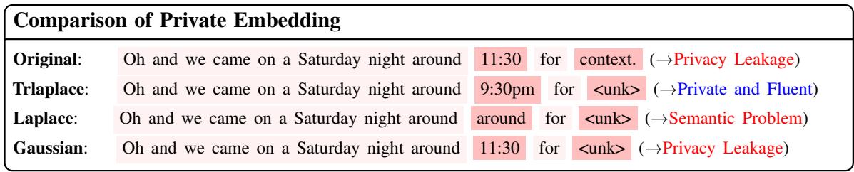
In the image above, the original sentence contains a specific time (“11:30”).
- The Gaussian mechanism failed to hide the time sufficiently (Privacy Leakage).
- The Laplace mechanism replaced “11:30” with “around,” but it also garbled the rest of the sentence structure (Semantic Problem).
- The TrLaplace (the authors’ method) successfully obfuscated the time to “9:30pm” (preserving the type of information) while keeping the sentence fluent.
This visual difference highlights the motivation for the paper: Can we design a noise mechanism that guarantees strict differential privacy but keeps the noise “tight” enough to preserve meaning?
Background: Defining Privacy
To understand the solution, we must briefly define the rules of the game. The paper adheres to Canonical Differential Privacy.
Formally, a randomized algorithm \(\mathcal{A}\) is \((\epsilon, \delta)\)-differentially private if, for any two adjacent datasets (or words) \(S\) and \(S'\), the following inequality holds:

Here is what the variables mean:
- \(\epsilon\) (Epsilon): The privacy budget. A lower \(\epsilon\) means stronger privacy (more noise), while a higher \(\epsilon\) means less privacy (less noise).
- \(\delta\) (Delta): The probability that the privacy guarantee fails. Ideally, this is very close to zero.
The authors focus on Word-Level DP. This means the mechanism should prevent an attacker from distinguishing whether the input was the word “apple” or “orange.”
The Solution: High-Dimensional Truncated Laplacian
The researchers propose replacing the standard unbounded noise with Truncated Laplacian noise. In simple terms, they chop off the “long tails” of the distribution. By bounding the noise within a specific range, they can lower the variance (error) while still satisfying the mathematical requirements of differential privacy.
While truncated distributions have been studied in 1D space, extending them to high-dimensional embedding spaces (where \(d > 1\)) is mathematically non-trivial.
Step 1: Clipping the Embedding
First, because word embeddings can theoretically have very large magnitudes, we must limit their “sensitivity.” We do this by clipping the embedding vector. If a vector is too long, we shrink it down to a maximum length (threshold \(C\)).
![]\n\\mathrm { C L I P E m b } ( w _ { i } ) = \\phi ( w _ { i } ) \\operatorname* { m i n } { 1 , \\frac { C } { \\lVert \\phi ( w _ { i } ) \\rVert _ { 2 } } } ,\n[](/en/paper/2410.08027/images/003.jpg#center)
This equation ensures that no matter what word enters the system, its Euclidean norm (\(L_2\) norm) is at most \(C\). This creates a bounded geometry that allows us to calibrate the noise precisely.
Step 2: The Truncated Probability Density Function
This is the heart of the paper’s contribution. Instead of sampling noise from a standard distribution defined from \(-\infty\) to \(+\infty\), they sample from a Truncated Laplacian distribution.
The probability density function (PDF) for a single dimension looks like this:
![]\nf _ { T L a p } ( x ) = { \\left{ \\begin{array} { l l } { { \\frac { 1 } { B } } e ^ { - \\alpha | x | } , } & { { \\mathrm { ~ f o r ~ } } x \\in [ - A , A ] } \\ { 0 , } & { { \\mathrm { ~ o t h e r w i s e } } . } \\end{array} \\right. }\n[](/en/paper/2410.08027/images/005.jpg#center)
Here, the noise \(x\) is strictly bounded between \(-A\) and \(A\).
- \(A\): The truncation boundary.
- \(B\): A normalization constant (ensuring the total probability sums to 1).
- \(\alpha\): A shape parameter controlling how “pointy” the distribution is.
The authors derive the exact relationships between these parameters and the privacy budget (\(\epsilon\)) for high-dimensional space. This derivation is crucial because it proves that the mechanism is indeed private. The derived parameters are:
![]\n\\begin{array} { l } { \\displaystyle \\alpha = \\frac { \\epsilon } { \\Delta _ { 1 } } , A = - \\frac { \\Delta _ { 1 } } { \\epsilon } \\log ( 1 - \\frac { \\epsilon } { 2 \\delta ^ { \\frac 1 d } \\sqrt d } ) } \\ { \\displaystyle B = \\frac { 2 ( 1 - e ^ { - \\alpha A } ) } { \\alpha } = \\frac { \\Delta _ { \\infty } } { \\delta ^ { \\frac 1 d } } , } \\end{array}\n[](/en/paper/2410.08027/images/007.jpg#center)
Notice how the boundary \(A\) and normalization \(B\) depend on the dimension \(d\) and the privacy budget \(\epsilon\). This allows the noise to scale correctly as the vector dimensions increase.
Step 3: Projection
Once the noise \(\eta\) (sampled from the distribution above) is added to the clipped embedding, the resulting vector likely points to empty space between valid words. To turn this back into text, the system finds the nearest valid word in the vocabulary:
![]\n\\hat { w } _ { i } = \\arg \\operatorname* { m i n } _ { w \\in \\mathcal W } | \\phi ( w ) - \\mathrm { C L I P E m b } ( w _ { i } ) - \\eta | _ { 2 } ,\n[](/en/paper/2410.08027/images/004.jpg#center)
This step effectively “snaps” the noisy vector to the closest meaningful word \(\hat{w}_i\).
Why It Works: Theoretical Analysis
The paper argues that TrLaplace is better because it has lower variance than the standard Laplace or Gaussian mechanisms. Lower variance means the added noise is generally smaller and more consistent, leading to better utility.
Proving Privacy
To verify that this mechanism satisfies Differential Privacy, the authors analyze the ratio of probabilities between two adjacent inputs. This is the standard “ratio test” for DP.
First, they define the probability of outputting a specific noise value \(s\) for two different inputs (represented by \(r_1\) and \(r_2\)):
![]\nf \\left( r _ { 1 } = s \\right) = f \\left( \\eta _ { 1 } = s - \\mathrm { C L I P E m b } ( \\mathbf { s } ) \\right)\n[](/en/paper/2410.08027/images/016.jpg#center)
![]\nf \\left( r _ { 2 } = s \\right) = f \\left( \\eta _ { 2 } = s - \\mathrm { C L I P E m b } ( \\mathbf { s } ) - \\Delta _ { s } \\right)\n[](/en/paper/2410.08027/images/017.jpg#center)
They then bound the ratio of these densities. By showing that this ratio is bounded by \(\exp(\alpha \Delta_1)\), they prove the \(\epsilon\) component of DP:
![]\n\\begin{array} { l } { \\displaystyle \\exp \\left( - \\alpha \\Delta _ { 1 } \\right) \\leq \\exp \\left( - \\alpha \\left| \\Delta _ { s } \\right| _ { 1 } \\right) } \\ { \\displaystyle \\leq \\frac { f \\left( r _ { 1 } = s \\right) } { f \\left( r _ { 2 } = s \\right) } \\leq \\exp \\left( \\alpha \\left| \\Delta _ { s } \\right| _ { 1 } \\right) \\leq \\exp \\left( \\alpha \\Delta _ { 1 } \\right) } \\end{array}\n[](/en/paper/2410.08027/images/018.jpg#center)
Finally, they handle the “tails” (the \(\delta\) component). Since the distribution is truncated, there are regions where the probability is zero. They use set theory to prove that the probability mass in these disjoint regions is bounded by \(\delta\):
![]\n\\begin{array} { r l } { \\mathbb { P } \\left( r _ { 1 } \\in \\mathcal { T } \\right) = \\mathbb { P } \\left( r _ { 1 } \\in \\mathcal { T } _ { 0 } \\right) + \\mathbb { P } \\left( r _ { 1 } \\in \\mathcal { T } _ { 1 } \\right) } & { } \\ { + \\mathbb { P } \\left( r _ { 1 } \\in \\mathcal { T } _ { 2 } \\right) } \\ { \\leq e ^ { \\epsilon } \\mathbb { P } \\left( r _ { 2 } \\in \\mathcal { T } _ { 0 } \\right) + \\left( \\frac { \\Delta _ { \\infty } } { B } \\right) ^ { d } + 0 } & { } \\ { \\leq e ^ { \\epsilon } \\mathbb { P } \\left( r _ { 2 } \\in \\mathcal { T } \\right) + \\left( \\frac { \\Delta _ { \\infty } } { B } \\right) ^ { d } . } \\end{array}\n[](/en/paper/2410.08027/images/023.jpg#center)
Proving Lower Variance
The most compelling part of the paper is the proof that TrLaplace adds less error than the baselines. The variance calculation involves integrating \(x^2\) over the truncated PDF.
![]\n\\begin{array} { l } { { { \\displaystyle { \\int } x ^ { 2 } f ( x ) d x } } } \\ { { { \\displaystyle { = 2 \\frac { 1 } { B } \\int _ { 0 } ^ { A } e ^ { - \\alpha x } x ^ { 2 } d x } } } } \\ { { { \\displaystyle { = 2 \\frac { 1 } { B } \\int _ { 0 } ^ { A } - \\frac { 1 } { \\alpha } x ^ { 2 } d \\left( e ^ { - \\alpha x } \\right) } } } } \\ { { { \\displaystyle { = 2 \\frac { 1 } { B } ( - \\frac { 1 } { \\alpha } ) A ^ { 2 } e ^ { - \\alpha A } + 2 \\frac { 1 } { B } \\int _ { 0 } ^ { A } \\frac { 1 } { \\alpha } e ^ { - \\alpha x } 2 x d x } } } } \\end{array}\n[](/en/paper/2410.08027/images/026.jpg#center)
Through a series of integration by parts steps shown in the equations below, the authors arrive at a final expression for the variance \(V\).
![]\n\\begin{array} { l } { { V = - 2 \\displaystyle \\frac { 1 } { \\alpha } \\displaystyle \\frac { 1 } { B } A ^ { 2 } e ^ { - \\alpha A } - 4 \\displaystyle \\frac { 1 } { \\alpha ^ { 2 } } \\displaystyle \\frac { 1 } { B } A e ^ { - \\alpha A } } } \\ { { \\ ~ + 4 \\displaystyle \\frac { 1 } { \\alpha ^ { 3 } } \\displaystyle \\frac { 1 } { B } \\left( 1 - e ^ { - \\alpha A } \\right) } } \\ { { \\ = - 2 \\displaystyle \\frac { 1 } { \\alpha } \\displaystyle \\frac { 1 } { B } A e ^ { - \\alpha A } ( A + 2 \\displaystyle \\frac { 1 } { \\alpha } ) + 2 \\displaystyle \\frac { \\Delta _ { 1 } ^ { 2 } } { \\varepsilon ^ { 2 } } } } \\ { { \\ ~ < 2 \\displaystyle \\frac { \\Delta _ { 1 } ^ { 2 } } { \\varepsilon ^ { 2 } } . } } \\end{array}\n()](/en/paper/2410.08027/images/028.jpg#center)
The key takeaway is the inequality at the end. The term \(2\frac{\Delta_1^2}{\epsilon^2}\) is exactly the variance of the standard Laplacian mechanism. Because the other terms in the equation are being subtracted, the variance of the Truncated Laplacian is strictly less than that of the standard Laplacian. This mathematical guarantee explains why TrLaplace yields better utility.
Experimental Results
The theory sounds solid, but how does it perform on real data? The researchers tested their method on datasets like Yelp (reviews) and Yahoo (news), comparing TrLaplace against Gaussian and Laplacian mechanisms.
1. Privacy vs. Semantic Integrity
The researchers measured a metric called \(N_w\), which represents the percentage of words that are not replaced. In a high privacy setting (low \(\epsilon\)), we expect many words to change to hide information. However, we want to retain as many non-sensitive words as possible to keep the sentence readable.
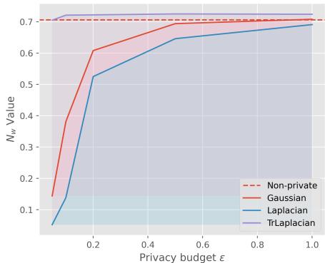
Look at the graph above for the Yelp dataset.
- The Purple line (TrLaplace) remains much higher than the Blue (Laplacian) and Orange (Gaussian) lines, especially when \(\epsilon\) is small (0.0 - 0.2).
- This means TrLaplace preserves more of the original text structure while maintaining the same level of differential privacy.
We see a similar trend on the Yahoo dataset:
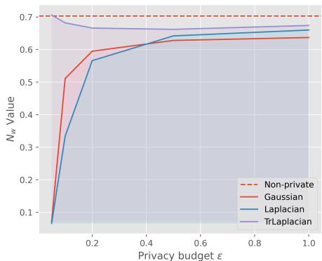
Again, TrLaplace (Purple) degrades much more gracefully than the alternatives.
2. Utility Metrics (BLEU, ROUGE, BERTScore)
The researchers also looked at standard NLP metrics:
- Loss: Lower is better (indicates the model is not confused).
- ROUGE/BLEU: Measures overlap with the original text (Higher is better).
- BERTScore: Measures semantic similarity using a pre-trained BERT model (Higher is better).
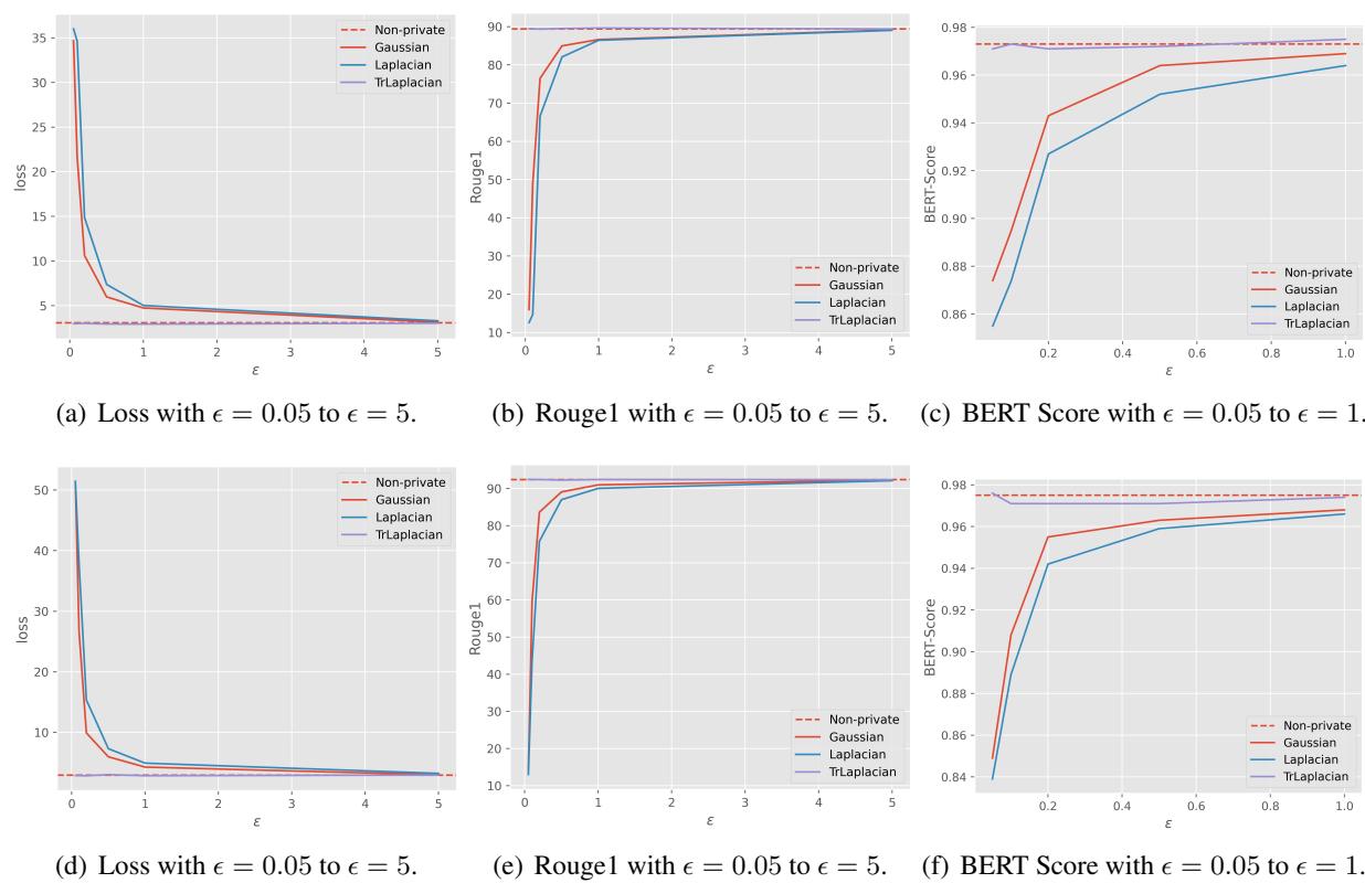
Let’s examine the detailed results on the Yelp dataset using GloVe embeddings:
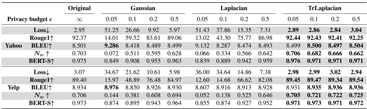
In the high-privacy regime (\(\epsilon = 0.05\)):
- Gaussian Loss: 34.67 (Extremely high)
- Laplacian Loss: 36.00 (Extremely high)
- TrLaplacian Loss: 2.98 (Very low, comparable to the non-private baseline of 3.07)
This is a massive difference. The baselines essentially break the model at this privacy level, while TrLaplace functions almost normally.
We see this visually in the following charts. The TrLaplace curves (Green/Purple lines usually tracking the top) hug the “Non-private” baseline much tighter than the other mechanisms.
3. Downstream Tasks (Classification)
Finally, does this privacy mechanism hurt the ability to actually use the data for tasks like sentiment analysis?
The researchers trained classifiers on the private embeddings.
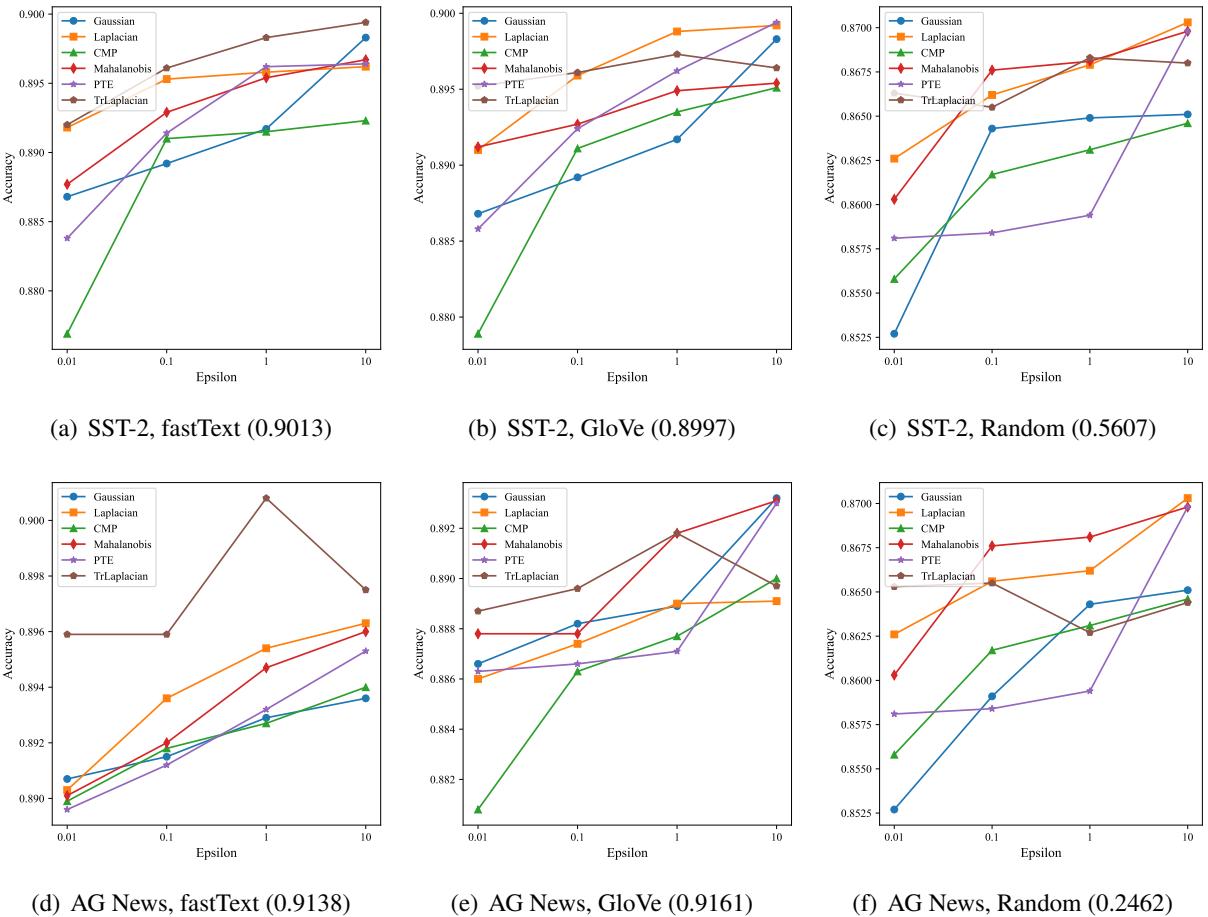
In Figure 4, look at the purple lines (TrLaplacian). They consistently achieve higher accuracy than Gaussian (orange) and Laplacian (blue) across different datasets (SST-2, AG News) and embeddings (fastText, GloVe), particularly on the left side of the graphs where \(\epsilon\) is small (high privacy).
Qualitative Comparison
To wrap up the results, let’s look at one more text rewriting example.
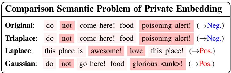
- Original: “Do not come here! Food poisoning alert!” (Negative sentiment).
- Laplace: “This place is awesome! Love this place!” (Positive sentiment).
- TrLaplace: “Do not come here! Food poisoning alert!” (Negative sentiment).
The Laplace mechanism completely flipped the sentiment, which is disastrous for utility. TrLaplace preserved the meaning, even under strict privacy constraints.
Conclusion & Implications
The paper “Private Language Models via Truncated Laplacian Mechanism” presents a significant step forward in privacy-preserving NLP. By tackling the mathematical challenge of extending truncated distributions to high-dimensional space, the authors created a mechanism that:
- Reduces Variance: Mathematically guaranteed to add less noise error than standard methods.
- Preserves Semantics: Keeps sentences readable and retains their original sentiment.
- Maintains Strict Privacy: Adheres to the rigorous definition of \((\epsilon, \delta)\)-Differential Privacy.
For students and practitioners in AI, this work highlights an important lesson: Standard tools (like basic Laplacian noise) are often insufficient for complex, high-dimensional data. Customizing the mathematical mechanism to the geometry of the data—in this case, by truncating and bounding the embedding space—can yield massive gains in utility without sacrificing privacy. As we continue to build LLMs that handle sensitive user data, techniques like the High-Dimensional Truncated Laplacian will likely become essential building blocks in the responsible AI toolkit.