Introduction

In the world of machine learning, the mantra “data is fuel” has become a cliché, but it remains fundamentally true. The characteristics of a training dataset—its quality, diversity, and hidden biases—dictate the capabilities of the final model. However, analyzing this “fuel” is notoriously difficult.

Currently, if a data scientist wants to understand their training data, they often look at attributes like “difficulty” (how hard is this sample to learn?) or “noisiness.” While useful, these metrics usually focus on individual instances in isolation. They fail to answer broader questions: How similar is Dataset A to Dataset B? Does this specific subset of 100 examples represent the knowledge of the entire dataset?

Enter RepMatch, a novel framework proposed by Modarres, Abbasi, and Pilehvar. Instead of analyzing data based on statistical properties of the text (like word counts or keyword overlap), RepMatch characterizes data through the lens of the model itself.

In this post, we will explore how RepMatch quantifies the similarity between arbitrary subsets of data by comparing the “knowledge” encoded in models trained on them. We will break down the clever use of Low-Rank Adaptation (LoRA) to make this comparison computationally feasible and look at how this method can be used to select better training data and detect dataset artifacts.

The Core Problem: Comparing Knowledge

Imagine you have two different textbooks. How do you determine if they cover the same material? You could count how many words overlap, but that’s superficial. A better way is to have a student read Book A and another student read Book B, and then compare what they have learned. If both students have acquired the same understanding of physics, we can say the books are “representationally similar.”

This is the philosophy behind RepMatch. The researchers define two subsets of data, \(S_1\) and \(S_2\), as similar if a model trained on \(S_1\) learns a representation space that aligns closely with a model trained on \(S_2\).

However, this creates a technical bottleneck. Modern Large Language Models (LLMs) have billions of parameters. Comparing two massive weight matrices directly is computationally expensive and statistically noisy. We need a way to isolate exactly what changed during training without getting lost in the noise of billions of parameters.

The Solution: LoRA and Grassmann Similarity

The researchers solved the comparison problem by combining two powerful concepts: Low-Rank Adaptation (LoRA) and Grassmann Similarity.

1. Constraining Updates with LoRA

Standard fine-tuning updates all the weights in a model. RepMatch, however, leverages LoRA (Hu et al., 2021). LoRA freezes the pre-trained model weights and injects small, trainable rank-decomposition matrices into each layer.

During training on a specific subset of data, only these small LoRA matrices are updated. This means that the “knowledge” gained from that specific subset is captured entirely within these compact low-rank matrices.

If we have a pre-trained weight matrix \(W\), the fine-tuned version is \(W + \Delta W\). In LoRA, this update \(\Delta W\) is the product of two small matrices, \(A\) and \(B\). RepMatch focuses on analyzing this \(\Delta W\), effectively isolating the task-specific features extracted from the data.

2. Measuring Similarity with Grassmannian Geometry

Once the researchers isolated the update matrices (\(\Delta W\)) for two different models, they needed a mathematical ruler to measure their similarity. They chose Grassmann similarity, a metric used to compare subspaces.

Conceptually, a low-rank matrix creates a specific geometric subspace. If two models have learned similar features, their update matrices should form subspaces that overlap significantly.

The mathematical formulation for this similarity measure \(\phi\) between two matrices \(W^r\) and \(W^{r'}\) is:

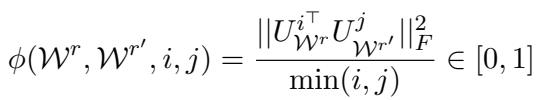
Here, \(U\) represents the singular vectors (obtained via Singular Value Decomposition, or SVD) of the update matrices. The equation essentially calculates how well the basis vectors of one subspace align with the basis vectors of the other. The result is a score between 0 (completely different) and 1 (identical subspaces).

Visualizing the Similarity

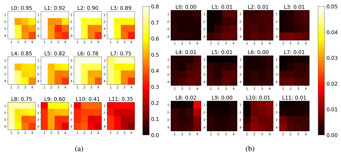
To prove this works, the authors visualized the similarity across the layers of a BERT model.

In the figure below, Panel (a) compares two models trained on the same dataset (SST-2) but with different random seeds. You can see the bright yellow blocks, indicating very high similarity scores (near 1.0 in some layers). This confirms that the metric is robust; even if the random seed changes, the model learns the same fundamental “knowledge.”

In contrast, Panel (b) compares a trained model against a “random baseline” (a shuffled matrix). The result is almost entirely black/red, with scores near 0.02. This sharp contrast validates that RepMatch is genuinely measuring learned structure, not random noise.

RepMatch in Action: Analysis Possibilities

The flexibility of RepMatch allows for two distinct types of analysis: Dataset-Level and Instance-Level. Because the method doesn’t care about the size of the subset, you can compare a single sentence to a whole dataset, or compare two massive datasets against each other.

Instance-Level Robustness

Before trusting the metric for complex tasks, we need to know if it works at the granular level of single examples.

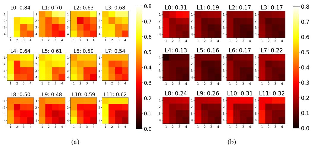
The researchers conducted an experiment where they fine-tuned models on a single instance of data.

• Figure 2a (below) shows the similarity between models trained on the same instance with different seeds. The scores are high (mostly yellow/orange).
• Figure 2b (below) shows the similarity between models trained on two different instances. The scores drop significantly (mostly red/black).

This confirms that RepMatch can distinguish the specific informational content of a single data point.

Dataset-Level Similarity

One of the most intuitive applications of RepMatch is comparing different datasets to see if they are “compatible” or cover similar tasks.

In the experiment below, the researchers compared the SST-2 dataset (Sentiment Analysis) against three others:

1. IMDB: Another sentiment analysis dataset.
2. SST-5: A fine-grained version of SST-2.
3. SNLI: A textual entailment dataset (completely different task).

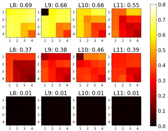
The results in Figure 3 (above) align perfectly with intuition:

• Middle Row (SST-2 vs. SST-5): High similarity (bright yellow). These datasets are essentially siblings.
• Top Row (SST-2 vs. IMDB): Moderate similarity. They share the same task (sentiment) but come from different domains (short phrases vs. movie reviews).
• Bottom Row (SST-2 vs. SNLI): Near-zero similarity (black). Sentiment analysis logic does not transfer to textual entailment logic.

This confirms that RepMatch successfully captures the semantic and task-level nature of the datasets.

Comparing Against Baselines

You might wonder, “Why not just compare the pre-trained embeddings of the data?” The authors tried this. They used a baseline that compares the Cosine Similarity of the [CLS] token representations of the raw data.

The results, shown in Table 2, highlight a critical failure of the baseline.

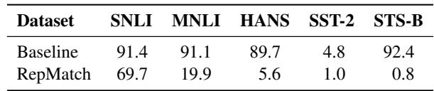
Notice the column for STS-B. The baseline method claims STS-B is 92.4% similar to SNLI. This is misleading; STS-B is a semantic similarity task, while SNLI is an inference task. They look similar on the surface (both involve pairs of sentences), so the pre-trained embeddings are similar. However, RepMatch correctly identifies that the knowledge required to solve them is different, giving a similarity score of only 0.8%.

Application 1: Data Efficiency (Training with Less)

Perhaps the most exciting application of RepMatch for students and practitioners is Data Selection.

If we can measure how similar a single instance is to the “ideal” knowledge of the full dataset, we can identify the most representative examples. The hypothesis is simple: training on a small subset of highly representative data should yield better results than training on a random subset.

The Experiment

1. Calculate the RepMatch score of every instance in a dataset against the full dataset.
2. Select the top 100 instances with the highest scores.
3. Train a BERT model on just those 100 instances.
4. Compare performance against a model trained on 100 random instances.

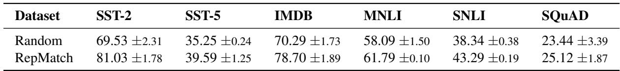
The Results

The results were consistent across multiple datasets. As shown in Table 1, the RepMatch-selected subsets consistently outperformed random selection. For the SST-2 dataset, the accuracy jumped from 69.53% (Random) to 81.03% (RepMatch).

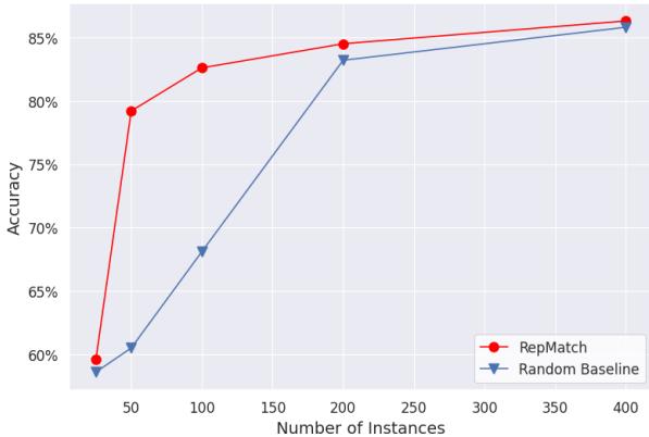
This advantage holds true even as the subset size grows. Figure 4 illustrates the performance curve on SST-2. While the gap narrows as more data is added (eventually, random selection catches enough good data by chance), RepMatch provides a massive “cold start” advantage when data or compute is limited.

Application 2: Detecting Dataset Artifacts

The final major contribution of the paper is using RepMatch to detect “out-of-distribution” instances and dataset artifacts.

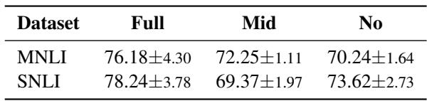
In Natural Language Inference (NLI) datasets, there is a known issue called the overlap bias. Models often cheat by assuming that if two sentences share many words, they “entail” each other. Challenge datasets like HANS were created to break this heuristic, containing examples with high word overlap that are actually not entailment.

The researchers hypothesized that bad training examples in standard NLI datasets (those that reinforce this cheating behavior) would be representationally similar to the HANS dataset.

To test this, they split the NLI data into three groups based on word overlap:

1. Full Overlap
2. Mid Overlap
3. No Overlap

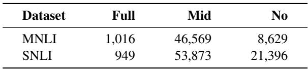
They then calculated the RepMatch score between these groups and the HANS dataset.

The results in Table 5 confirm the hypothesis. The “Full Overlap” subset had the highest similarity to HANS. This means RepMatch successfully identified the specific subset of training data that relied on the overlap heuristic. This capability is incredibly powerful for debugging datasets and improving out-of-distribution generalization.

Conclusion and Future Implications

RepMatch represents a significant shift in how we analyze datasets. By moving away from surface-level statistics and measuring the change in model representation, we gain a much deeper understanding of what our models are actually learning.

The key takeaways from this research are:

1. Low-Rank Adaptation (LoRA) serves as an efficient vessel for capturing task-specific knowledge.
2. Grassmann Similarity provides a robust mathematical framework for comparing these knowledge states.
3. Practical Utility: RepMatch isn’t just theoretical. It effectively selects high-quality training data (beating random sampling) and uncovers hidden biases and artifacts in standard datasets.

For students and researchers, this opens up new avenues for “Data-Centric AI.” Instead of just building bigger models, we can use tools like RepMatch to curate smarter, more efficient datasets, leading to models that learn faster and generalize better. As we continue to rely on massive, opaque datasets to train our AI, having a tool that lets us see through the model’s eyes is invaluable.