Why LLMs Struggle with Uncertainty: Inside the QUITE Benchmark and the Neuro-Symbolic Solution

Introduction

We often treat Large Language Models (LLMs) like omniscient reasoning engines. We feed them complex scenarios, legal documents, or medical summaries and ask them to derive conclusions. But how good are these models really when the answers aren’t black and white?

In the real world, certainty is a luxury. A doctor doesn’t say “This symptom always means X.” They say, “Given this symptom, the diagnosis is highly likely to be X, unless Y is also present.” This is probabilistic reasoning—the ability to handle uncertainty, weigh evidence, and update beliefs.

A recent paper titled “QUITE: Quantifying Uncertainty in Natural Language Text in Bayesian Reasoning Scenarios” investigates this exact capability. The researchers created a challenging dataset to test whether LLMs can truly reason with probability or if they are just mimicking the patterns of logic.

The findings are eye-opening: while LLMs are eloquent, their ability to perform complex probabilistic reasoning—especially “backward” reasoning—is severely limited. However, the paper also offers a solution: a neuro-symbolic approach that combines the linguistic fluency of LLMs with the rigorous logic of probabilistic programming.

The Background: Bayesian Networks and How We Reason

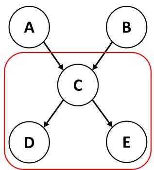
To understand the challenge, we first need to understand the tool scientists use to model these problems: the Bayesian Network.

A Bayesian Network is a graph where nodes represent random variables (events) and arrows represent dependencies (probabilities). For example, “Rain” influences “Wet Grass.” Associated with these nodes are probability tables that tell us exactly how likely an event is given its parents.

The paper identifies three distinct types of reasoning we perform on these networks, as illustrated below:

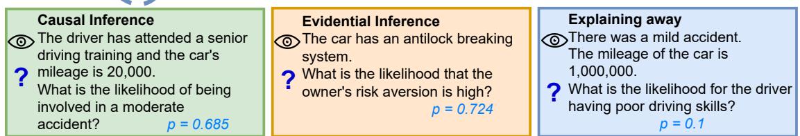
1. Causal Inference (Forward): We observe a cause and predict the effect.

• Example: You see a driver with “adventurous” behavior (Cause). What is the probability of an accident (Effect)?
• Status: Humans and machines generally find this intuitive.

2. Evidential Inference (Backward): We observe an effect and infer the cause.

• Example: You see a car has anti-lock brakes (Effect). What is the probability the owner is risk-averse (Cause)?
• Status: This requires applying Bayes’ theorem to “invert” the probabilities. It is computationally harder.

3. Explaining-Away: This occurs when two independent causes share a common effect.

• Example: A “Mild Accident” (Effect) could be caused by “Bad Driving” or “Bad Weather.” If we learn the weather was terrible, the probability that the driver has bad skills goes down (the weather “explains away” the accident).
• Status: This is a sophisticated cognitive leap that requires understanding the interplay between multiple variables.

The Problem with Current Benchmarks

Previous attempts to test LLMs on these tasks have been too simple. They often used:

• Binary variables only: (True/False). Real life has categories (High/Medium/Low).
• Numeric-only inputs: “There is a 70% chance.” Real humans use language.
• Simple Templates: Sentences that look like code, which LLMs can game easily.

The QUITE dataset (Quantifying Uncertainty in Natural Language Text) changes this. It uses real-world networks from domains like medicine and car insurance, includes categorical variables, and crucially, introduces Words of Estimative Probability (WEPs).

Words of Estimative Probability (WEPs)

In natural conversation, we rarely speak in exact percentages. We use words like “likely,” “improbable,” or “almost certain.” To simulate this, the researchers mapped probabilities to specific adverbs based on human perception studies.

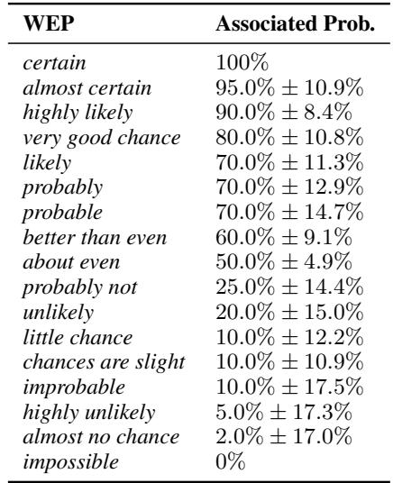
This adds a layer of difficulty: the model must first interpret the linguistic nuance (“better than even” \(\approx\) 60%) before it can even attempt the mathematical reasoning.

The QUITE Dataset Construction

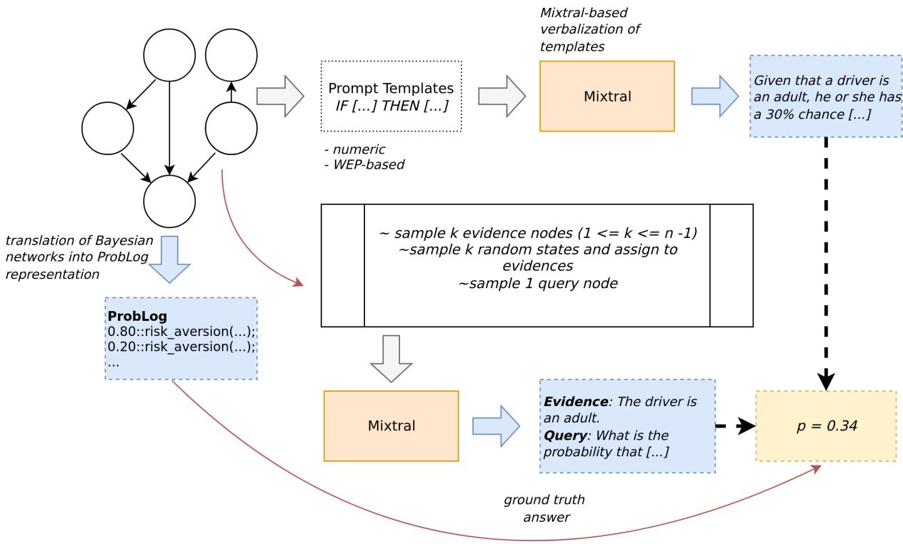
The researchers built QUITE by taking established Bayesian networks and verbalizing them. They didn’t just use templates; they used LLMs (specifically Mixtral) to generate rich, varied natural language descriptions of the relationships and probabilities.

The generation pipeline ensures that the text accurately reflects the complex mathematical dependencies of the original networks.

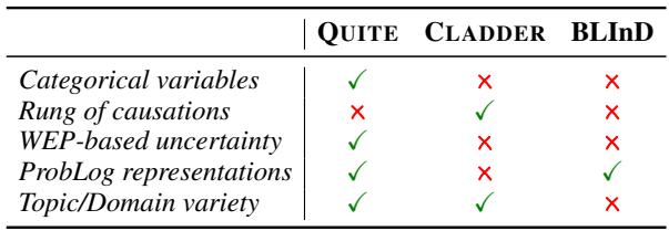
This process resulted in a dataset that is significantly more complex and linguistically diverse than predecessors like CLADDER or BLInD. As shown in the comparison below, QUITE is the only benchmark combining categorical variables, WEP-based uncertainty, and ProbLog representations.

The Core Method: Neuro-Symbolic vs. LLMs

The paper sets up a showdown between two distinct approaches to solving these reasoning problems.

Approach 1: Pure LLM Prompting

The researchers tested models like GPT-4, Llama-3, and Mixtral. They used:

• Zero-Shot: Simply giving the model the text and asking for the probability.
• Causal Chain-of-Thought (CoT): Asking the model to “think step-by-step,” write down the variables, and perform the calculation.

Approach 2: The Neuro-Symbolic Approach

This is the novel contribution. Instead of asking the LLM to do the math, they ask the LLM to write code that represents the math.

They fine-tuned a Mistral-7B model to act as a semantic parser. Its job is to read the natural language premises (e.g., “If the patient has gallstones, flatulence is likely”) and translate them into ProbLog, a probabilistic logic programming language.

Once the text is converted into the structured code seen above (Figure 4), a deterministic solver executes the program. This outsources the “reasoning” and “calculation” to a system guaranteed to be mathematically correct, leaving the LLM to do what it does best: understand language.

A Deep Dive: Why the Math is Hard

To appreciate why pure LLMs struggle, let’s look at the actual math required for a “simple” evidential reasoning query in the dataset.

Imagine a network with three variables: Gallstones, Flatulence, and Amylase levels. The model receives text describing the probabilities. It is then asked: “What is the likelihood of a patient having Amylase levels between 500-1400 given they have Flatulence?”

Mathematically, we need to calculate:

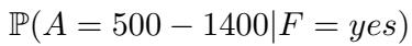
Using Bayes’ theorem, this expands to:

The problem is that the numerator (top part) isn’t given directly in the text. The model must “marginalize out” the Gallstones variable. It has to sum the probabilities for both the case where Gallstones are present and where they are not:

The model then has to find these values by multiplying the conditional probabilities hidden in the text. For the case where Gallstones are present (\(G=yes\)):

And for where they are absent (\(G=no\)):

Summing those gives the numerator:

But we aren’t done. We still need the denominator: the total probability of Flatulence (\(P(F=yes)\)). This requires marginalizing over all states of Gallstones and Amylase. Because Amylase is categorical with 3 states and Gallstones is binary, there are \(2 \times 3 = 6\) combinations to sum up!

![] = \mathbb { P } ( F = y e s , G = y e s , A = 0 - 2 9 9 )

• \mathbb { P } ( F = y e s , G = y e s , A = 3 0 0 - 4 9 9 ) [](images/022.jpg#center) (…plus 4 more terms…)

Finally, we divide the numerator by the denominator to get the final answer:

The takeaway: This is a massive amount of arithmetic context management. Expecting an LLM to hold all these numbers in its “head,” perform floating-point multiplication perfectly, and sum them up correctly without a calculator is asking for failure. The Neuro-symbolic approach avoids this entirely by simply writing the logic into code and letting the computer handle the math.

Experiments and Results

So, how did they compare? The results confirm that standard LLMs, even powerful ones like GPT-4, are not reliable probabilistic reasoners.

The Failure of Backward Reasoning

The most striking result is the breakdown of performance by reasoning type.

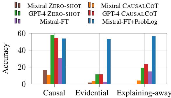
In Figure 1 above, look at the Causal column. GPT-4 (green/red bars) performs decently, getting over 50% accuracy. This makes sense; predicting effects from causes is similar to how text generation works (next-token prediction).

However, look at the Evidential and Explaining-away columns. The pure LLM approaches collapse, dropping to near zero or very low accuracy. They cannot effectively “reverse” the causal flow.

In contrast, the Mistral-FT+ProbLog (blue bar) remains robust across all three types. Because it translates the problem into a global logical structure, the direction of reasoning doesn’t matter to the solver. It handles backward inference just as easily as forward inference.

Error Analysis: Complexity Matters

The researchers also analyzed what causes the models to fail. Unsurprisingly, the size of the network (amount of context) plays a huge role.

For the Neuro-symbolic model (ProbLog-FT), performance is excellent for smaller networks but degrades as the text gets longer (more premises to parse).

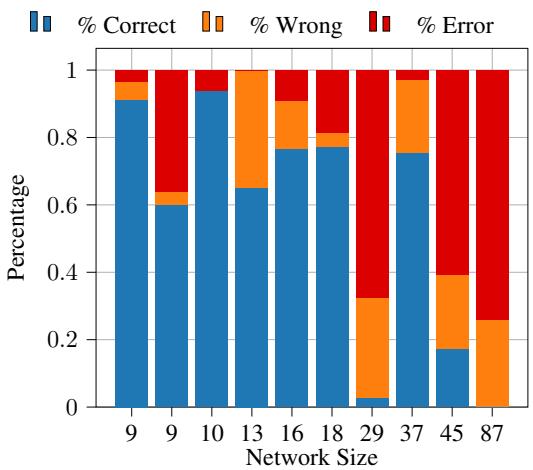
However, when we look at the pure LLM approach (GPT-4 with Causal Chain of Thought), the degradation is much more severe and chaotic. Even at moderate sizes, the error rate (red) explodes.

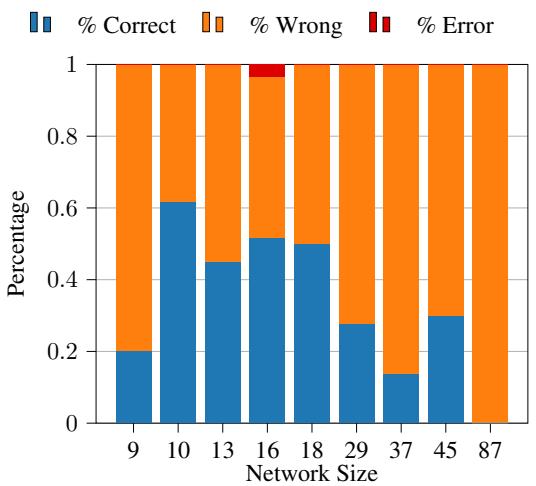
The primary errors for the LLMs were mathematical: rounding errors, wrong formulas, or simply hallucinating numbers. The primary errors for the Neuro-symbolic approach were parsing errors: generating invalid code. Interestingly, an “oracle” experiment showed that if the parsing is correct, the answer is guaranteed to be correct.

Conclusion

The QUITE paper provides a reality check for the reasoning capabilities of Large Language Models. It demonstrates that while LLMs understand the concept of causality, they struggle significantly with the rigorous, quantitative manipulation of uncertainty required for real-world Bayesian reasoning. They are particularly bad at evidential (backward) reasoning, which is often what we need most in fields like medical diagnosis or debugging.

The work strongly supports the case for Neuro-symbolic AI. By using LLMs as translators—converting messy, uncertain natural language into clean, structured code—and using classical solvers for the heavy lifting, we can build systems that are both flexible and logically sound.

As we move forward, the path to smarter AI might not be bigger language models, but language models that know how to use calculators and logic solvers.