The Ensemble Illusion: Why Deep Ensembles Might Just Be Large Models in Disguise

In the classical era of machine learning, “ensembling” was the closest thing to a free lunch. If you trained a single decision tree, it might overfit. But if you trained a hundred trees and averaged their predictions (a Random Forest), you got a robust, highly accurate model. The intuition was simple: different models make different mistakes, so averaging them cancels out the noise.

However, modern deep learning operates in a different regime: overparameterization. We now routinely train neural networks with far more parameters than training data points. Interestingly, practitioners still use ensembles (Deep Ensembles), claiming they improve accuracy and provide better uncertainty estimates.

But do the old intuitions hold up in this new world?

A recent paper, Theoretical Limitations of Ensembles in the Age of Overparameterization, challenges the conventional wisdom. The authors argue that in the overparameterized regime, ensembles don’t possess the same magical variance-reduction properties as they do in classical learning. Instead, an infinite ensemble of overparameterized models is mathematically equivalent to a single, larger model.

In this post, we will deconstruct this paper, exploring why adding more models to an ensemble might effectively be the same as just making your single model wider.

The Shift: From Underparameterized to Overparameterized

To understand the authors’ argument, we must first distinguish between the two regimes of machine learning.

1. Underparameterized (Classic): You have more data than parameters (e.g., linear regression on a tall dataset). The model cannot fit the training data perfectly (non-zero training error). Here, ensembling helps by reducing variance and stabilizing predictions.
2. Overparameterized (Modern): You have more parameters than data (e.g., deep neural networks). The model has enough capacity to memorize the training set perfectly (zero training error).

The authors use Random Feature (RF) models as a proxy to study this. RF models are a tractable approximation of neural networks. An RF model fixes the weights of the hidden layers and only trains the last linear layer.

The core question of the paper is: Does an ensemble of overparameterized models generalize better than a single, very large model trained on the same data?

The Core Equivalence

The paper’s most significant theoretical contribution is proving that, under minimal assumptions, an infinite ensemble of overparameterized models makes the exact same predictions as a single infinite-width model.

Visualizing the Equivalence

Let’s look at the behavior of Random Feature models. In the figure below, the left panel shows 100 individual finite-width models (blue lines) trained on a simple dataset. They vary wildly. However, the right panel shows what happens when you average 10,000 of them (an “infinite” ensemble).

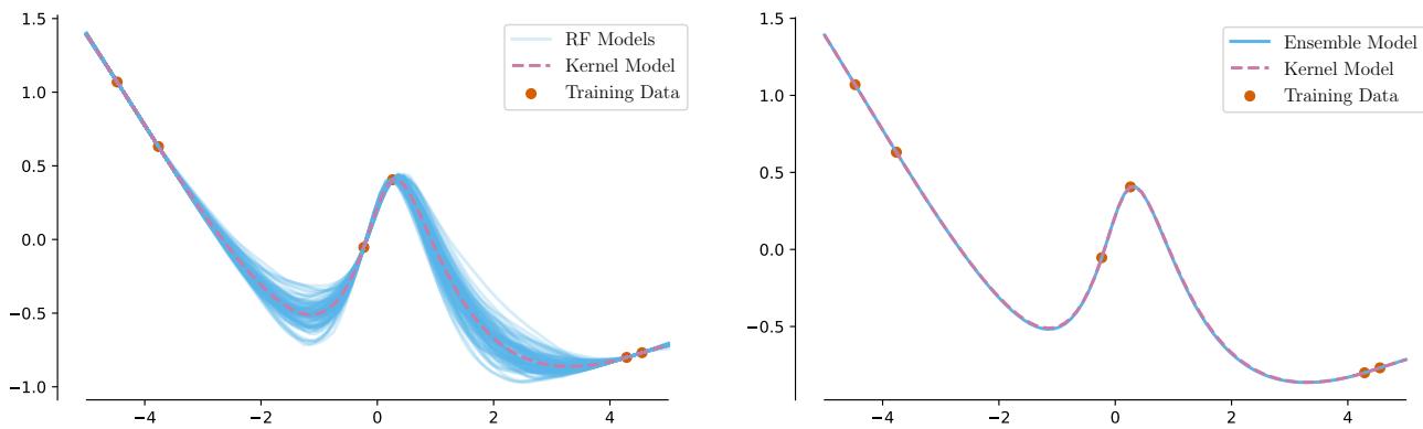
As you can see in the right panel, the ensemble prediction (blue) becomes indistinguishable from the single infinite-width model (pink). The authors prove that this isn’t a coincidence—it is a mathematical identity.

The Mathematics of Equivalence

To prove this, the authors analyze the “Ridgeless” Least Norm (LN) predictor. When a model is overparameterized, there are infinite solutions that fit the data perfectly. The “Least Norm” solution is the one that fits the data while keeping the weights as small as possible (which gradient descent tends to find).

The prediction of a single model with random features \(\mathcal{W}\) is denoted as \(h_{\mathcal{W}}^{(\mathrm{LN})}\). As the width \(D\) goes to infinity, this single model converges to a kernel predictor:

Now, consider an ensemble. An ensemble averages the predictions of many such models. The authors derive a decomposition for the prediction of an infinite ensemble, \(\bar{h}_{\infty}^{(LN)}(x^*)\), shown below:

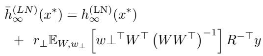
This equation is dense, so let’s break it down:

1. Term 1: \(h_{\infty}^{(LN)}(x^*)\) is the prediction of the single infinite-width model.
2. Term 2: The second part of the equation (starting with \(r_\perp\)) represents the difference between the ensemble and the single infinite model.

The variable \(W\) represents the random features projected onto the training data, and \(w_\perp\) represents the components of the features orthogonal to the data.

The Crucial Proof: The authors prove that the expected value in the second term is zero (under mild assumptions about the feature distribution).

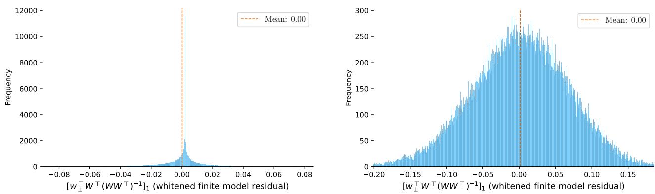
The histograms above (Figure 12) empirically validate this proof. Whether using ReLU or Gaussian Error features, the error term distributes perfectly around zero.

Conclusion: Since the error term vanishes, the infinite ensemble prediction is pointwise equivalent to the single infinite-width prediction. Ensembling adds no “new” function space coverage that a single giant model doesn’t already possess.

Finite Budgets: Ensembles vs. Giant Models

You might argue, “I can’t train an infinite-width model. I have a finite memory budget.”

The researchers addressed this by comparing two practical setups with the same total parameter budget:

1. Ensemble: \(M\) models, each with \(D\) features.
2. Single Large Model: 1 model with \(M \times D\) features.

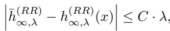
If classic intuition held, the ensemble should generalize better. However, the theoretical bound derived in the paper suggests otherwise:

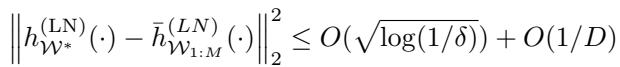
This inequality states that the squared difference between the large single model and the ensemble scales with \(O(1/D)\). As the individual models in the ensemble become sufficiently overparameterized (large \(D\)), the ensemble and the single giant model become nearly identical.

Empirical Results

The authors tested this on both Random Feature models and real Neural Networks (MLPs).

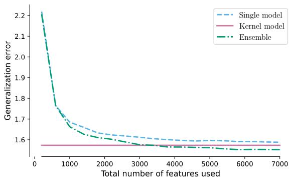
In Figure 3 above:

• Left (RF Models): The Green line (Ensemble) and Light Blue line (Single Large Model) track almost perfectly as the feature count increases.
• Right (Neural Networks): The same trend appears. The ensemble offers no significant generalization benefit over the single large model when the total parameter count is fixed.

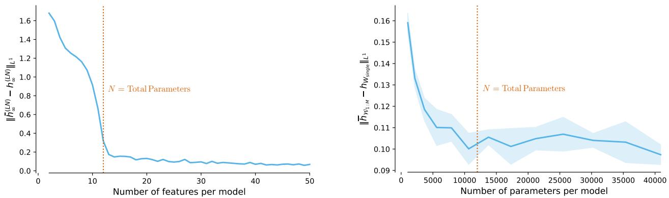
This creates a “Hockey Stick” pattern (Figure 2, below), where the difference between the two approaches is high when models are small (underparameterized), but collapses to zero once the models become overparameterized (\(D > N\)).

Rethinking Uncertainty and Variance

One of the main reasons practitioners use Deep Ensembles is for uncertainty quantification. The logic is: “If my ensemble members disagree (high variance), the model is uncertain.”

In Bayesian statistics, variance often correlates with “epistemic uncertainty” (uncertainty due to lack of data). However, the authors show that in the overparameterized regime, ensemble variance measures something else entirely.

The Variance Equation

The authors derive the predictive variance of the ensemble:

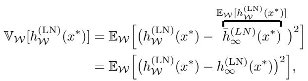
This equation shows that the variance is simply the expected squared difference between a finite-width model and the infinite-width limit. In plain English: Ensemble variance quantifies the expected change in prediction if we were to increase the model capacity.

It is a measure of sensitivity to parameterization, not necessarily a measure of how far you are from the training data.

The Gaussian Trap

Previous theoretical works assumed that random features are Gaussian. If you make that assumption, the math simplifies to a very specific form:

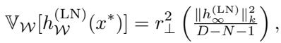
In this specific Gaussian case, the variance term \(r_\perp^2\) (shown below) actually does look like a Bayesian Gaussian Process posterior variance.

However, neural network features (like ReLU) are not Gaussian. When the authors analyzed general features, they found that the ensemble variance behaves very differently from the “ideal” Bayesian uncertainty.

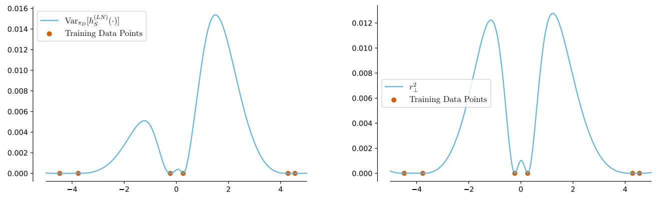
Look at Figure 4 (above).

• Left: The actual variance of an overparameterized ensemble.
• Right: The “ideal” Bayesian uncertainty (Gaussian Process posterior).

They look completely different. The peaks and troughs do not align. This suggests that using deep ensemble variance as a proxy for “I don’t know” might be misleading in safety-critical applications. It does not capture the distance from the training data in the way a Gaussian Process does.

Robustness to Regularization

The analysis above focuses on “ridgeless” regression (pure interpolation). Does this hold if we add regularization (Ridge Regression)?

The authors prove that the transition is smooth. They show that the difference between the ensemble and the single model is Lipschitz continuous with respect to the ridge parameter \(\lambda\).

This means that for small regularization (which is common in deep learning), the equivalence still holds approximately. As \(\lambda \to 0\), the difference vanishes.

Conclusion and Implications

The paper Theoretical Limitations of Ensembles in the Age of Overparameterization provides a sobering reality check for deep learning practitioners.

Key Takeaways:

1. The “Magic” is Capacity: The performance boost from Deep Ensembles largely comes from the fact that they are approximating a much larger single model. If you could train that larger model directly, you would likely get similar results.
2. No Free Lunch for Generalization: Once your component models are overparameterized, ensembling does not provide a fundamental generalization advantage over a single model with the same total parameter count.
3. Uncertainty Warning: Be careful interpreting ensemble variance as “uncertainty.” It primarily measures the model’s sensitivity to its own width/capacity, which may not align with true epistemic uncertainty (what the model doesn’t know).

Does this mean we should stop using ensembles? Not necessarily. Training one giant model is often harder (optimization difficulties) or computationally infeasible (memory constraints) compared to training \(M\) smaller models in parallel. Ensembles remain a practical computational hack.

However, we should stop viewing them as a distinct statistical method that provides “diversity” in the classical sense. In the age of overparameterization, an ensemble is just a distributed way of building a giant neural network.