Performing Brain Surgery on BERT: How to Locate and Edit Gender Bias in Language Models

Large Language Models (LMs) are mirrors of the data they are trained on. Unfortunately, this means they often reflect the societal biases, including gender stereotypes, found in the vast text of the internet. While we have many tools to measure this bias—checking if a model associates “doctor” more with men than women—we still have a limited understanding of where this bias physically lives inside the model. Which specific numbers (weights) among the millions or billions of parameters are responsible for thinking that “nurse” implies “female”?

In a recent paper, Local Contrastive Editing of Gender Stereotypes, researchers from the University of Mannheim, University of Amsterdam, and University of Hamburg propose a novel method to answer this question. They introduce Local Contrastive Editing, a technique that acts like microsurgery for neural networks. It allows us to pinpoint the exact subset of weights responsible for encoding stereotypes and, crucially, edit them to mitigate that bias without retraining the whole model.

In this post, we will break down how this method works, the mathematics behind it, and what the experiments reveal about the anatomy of bias in Artificial Intelligence.

The Challenge: Finding the Needle in the Haystack

To fix a problem, you usually need to know where it is. In the context of Deep Learning, this is the challenge of interpretability. A model like BERT has 110 million parameters. Modifying all of them (fine-tuning) is computationally expensive and risks “catastrophic forgetting,” where the model learns new rules but forgets how to speak English properly.

The researchers’ goal was twofold:

1. Localization: Identify the specific weights that drive stereotypical gender bias.
2. Modification: Change only those weights to steer the model’s behavior, reducing bias while keeping the rest of the model’s knowledge intact.

The Solution: Local Contrastive Editing

The core insight of this paper is that bias is best identified through contrast. Instead of looking at a single model in isolation, the researchers compare a Target Model (the one we want to fix) against a Reference Model (a model that behaves differently regarding the property we care about).

As illustrated below, the process is a two-step approach.

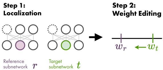
Step 1: Localization via Pruning

How do we determine which weights are “stereotypical”? The researchers utilized a technique called Iterative Magnitude Pruning (IMP), often associated with the “Lottery Ticket Hypothesis.”

The idea is to train a model and then remove (prune) the weights that have the smallest magnitude (values closest to zero), assuming they are the least important. If you do this repeatedly, you end up with a “sparse subnetwork”—a skeleton of the original model that still performs the task well.

The researchers discovered that if you create a “Stereotypical Subnetwork” and an “Anti-Stereotypical Subnetwork,” they will mostly look the same. However, a tiny fraction of weights will behave differently. These differences are where the bias hides.

They proposed two methods to identify these specific weights:

1. Mask-based Localization

This method looks at the structure of the subnetworks. A “mask” is a binary grid that says which weights are kept (1) and which are pruned (0). The researchers hypothesized that weights present in one model but pruned in the other are likely responsible for their different behaviors regarding gender.

They calculate a localization mask \(b\) by looking for the difference between the target mask (\(m_t\)) and the reference mask (\(m_r\)):

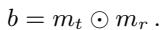
In simple terms: We are looking for the weights that are turned “on” in the reference model but “off” in the target model (or vice versa).

2. Value-based Localization

This method looks at the actual numerical values of the weights. Even if both models keep the same weight, the value of that weight might differ drastically. The researchers select the top-\(k\) weights with the largest absolute difference between the target and reference models.

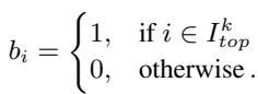
Here, \(I_{top}^k\) represents the indices of the weights where the reference and target disagree the most.

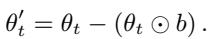
Step 2: Editing Strategies

Once the specific weights responsible for bias are identified (localized), the next step is to edit them. The researchers explored several mathematical operations to transform the weights of the target model (\(\theta_t\)) using the information from the reference model (\(\theta_r\)).

Figure 2 provides a visual summary of how these localization and editing strategies interact.

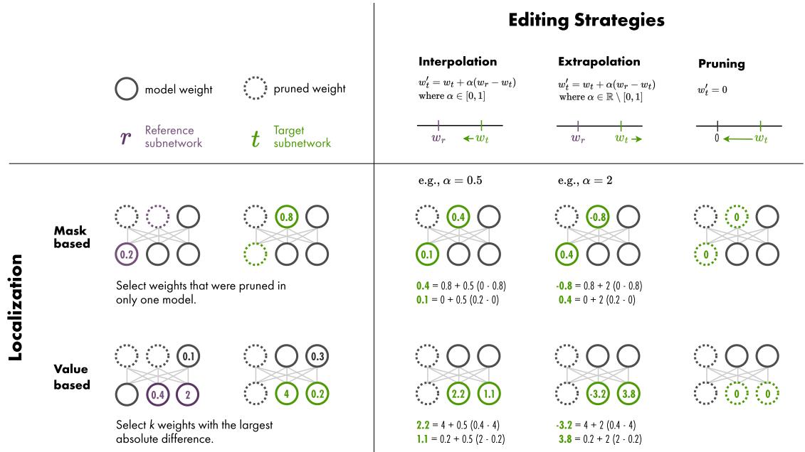
Let’s look at the specific editing formulas used:

Weight Interpolation (IP): This moves the target weights closer to the reference weights. If \(\alpha=0.5\), the new weight is exactly halfway between the stereotypical and anti-stereotypical versions. If \(\alpha=1\), the target simply adopts the reference weight.

Weight Extrapolation (EP): This is where it gets interesting. We can use a value of \(\alpha\) greater than 1 or less than 0. This allows us to push the model further in the direction of the reference, or even in the opposite direction, exaggerating the difference.

Pruning (PR): This strategy simply sets the identified “biased” weights to zero, effectively removing them from the calculation.

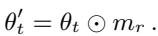
Mask Switch (SW): Specific to mask-based localization, this applies the reference model’s mask to the target model.

Experimental Setup: Creating “Sexist” BERT

To test if this works, the researchers needed clear test cases. They took the standard BERT model and fine-tuned it on Wikipedia data that had been artificially altered using Counterfactual Data Augmentation.

1. Stereotypical Model: Fine-tuned on data where gender associations were enforced (e.g., “The nurse… she”).
2. Anti-Stereotypical Model: Fine-tuned on data where associations were swapped (e.g., “The nurse… he”).
3. Neutral Model: Fine-tuned on unaltered data (for control).

They then measured bias using standard benchmarks like WEAT (Word Embedding Association Test), StereoSet, and CrowS-Pairs.

Did they find the bias?

Yes. The localization step revealed that the weights responsible for gender bias are not randomly distributed. As shown in Figure 3, the selected weights (colored bars) tend to cluster in specific components, particularly in the output dense layers of the attention mechanism in the deeper layers of the network.

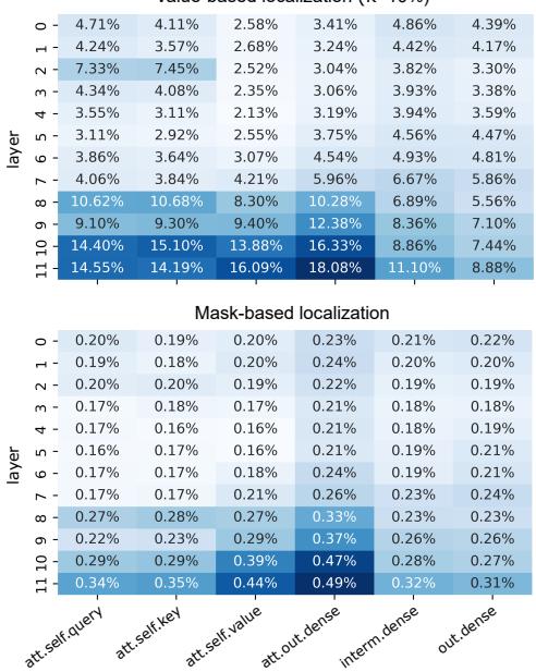
Crucially, less than 0.5% of the total weights were identified as relevant. This confirms that bias is not a holistic property of the entire “brain” of the model, but rather localized to specific connections.

Key Results: Controlling the Bias

The most exciting result of the paper is the demonstration of control. By editing just this tiny subset of weights (<0.5%), the researchers were able to steer the bias of the model significantly.

In the figure below, the x-axis represents the bias score (WEAT).

• Blue lines represent a Stereotypical Target model being edited toward an Anti-Stereotypical Reference.
• Red lines represent an Anti-Stereotypical Target being edited toward a Stereotypical Reference.

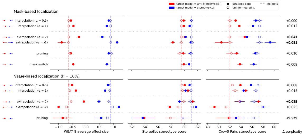
Takeaways from the results:

1. It Works: The blue lines move left (reducing bias) and the red lines move right (increasing bias) as the editing intensity (\(\alpha\)) increases.
2. Localization Matters: The white circles represent “uninformed edits”—randomly selecting weights to edit. Notice that these points barely move. This proves that you cannot just edit any weights; you must find the specific ones responsible for the stereotype.
3. Extrapolation Power: By using extrapolation (e.g., \(\alpha=2\)), the researchers could push a stereotypical model past the “neutral” point and turn it into an anti-stereotypical one.

Does the model still work?

A common fear with model editing is breaking the model’s ability to understand language (perplexity). If you remove the concept of “gender,” does the model forget what a “person” is?

The researchers tested this sensitivity. Figure 6 (b) shows the change in perplexity (y-axis) as the weighting factor (\(\alpha\)) changes.

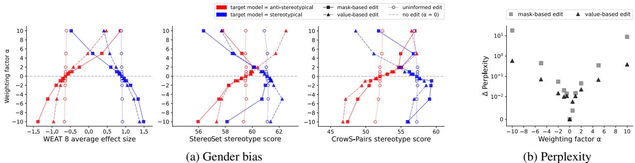
For most strategies, the change in perplexity is negligible (the dots stay near zero). However, Value-based Pruning (removing the weights with the largest value differences) caused a massive spike in perplexity (see the black triangles shooting up in 6b). This suggests that while those weights contain bias, they are also critical for the general function of the model. Interpolation and Extrapolation, however, proved to be safe and effective.

Applying to Neutral Models

Finally, the researchers applied this to a “Neutral” model—one that hadn’t been artificially forced to be sexist or anti-sexist. Could they reduce the natural bias present in a standard model?

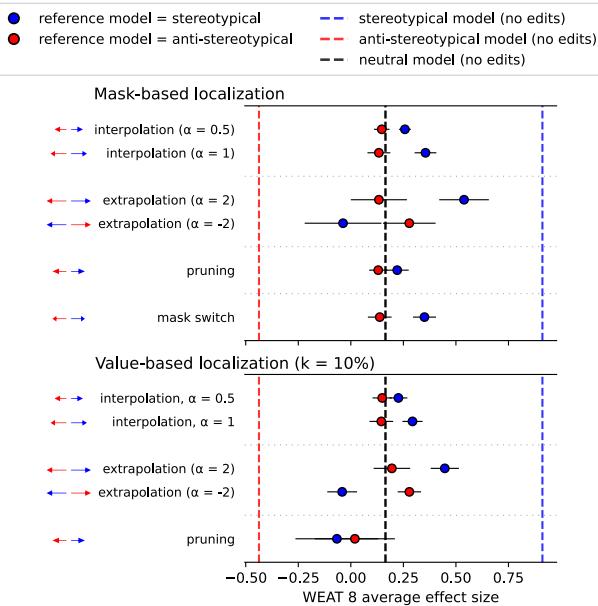
As shown in Figure 7, using a Stereotypical Reference model allowed them to identify and “subtract” bias from the Neutral model (using negative extrapolation, \(\alpha = -2\), shown in blue). This confirms the technique is applicable to real-world scenarios, not just artificially created test beds.

Conclusion

The paper “Local Contrastive Editing of Gender Stereotypes” offers a compelling step forward in AI safety. It moves us from simply observing bias to actively performing surgery on it.

Key Takeaways:

• Bias is Local: Stereotypes are encoded in a very small subset (<0.5%) of the model’s parameters, largely in the deeper attention layers.
• Contrast is Key: We can find these parameters by comparing a model to its “opposite” (a reference model).
• Editability: We can interpolate or extrapolate these weights to smoothly steer the model’s gender bias without retraining the whole network or destroying its language capabilities.

This method opens up new avenues for “parameter-efficient” bias mitigation. Instead of massive retraining pipelines, future developers might simply download a “patch”—a tiny set of weight adjustments—that corrects specific societal biases in their Large Language Models.