Why Random Sampling Isn’t Enough: The Power of Active Learning in Solving PDEs

If you have ever dabbled in scientific computing or machine learning for physics, you know the drill. You have a Partial Differential Equation (PDE), like the Heat equation or the Navier-Stokes equation, that describes a physical system. Traditionally, solving these requires heavy numerical solvers that chew up computational resources.

Enter Operator Learning. The goal here is to train a machine learning model to approximate the “solution operator” of the PDE. Instead of solving the equation from scratch every time, you feed the initial conditions or source terms into a neural network (or another estimator), and it spits out the solution almost instantly.

But there is a catch. To train these models, you need data—lots of input-output pairs. The standard approach, borrowed from classical statistical learning, is passive data collection: you generate random inputs, run your expensive solver to get the outputs, and train on that dataset.

A recent research paper, “On the Benefits of Active Data Collection in Operator Learning,” asks a fundamental question: Is random sampling actually the best way to learn these operators?

The answer is a resounding “No.” In this post, we will dive deep into this paper to understand why letting the learner choose its data (Active Learning) can lead to exponentially faster convergence rates compared to the traditional passive approach.

The Setup: Learning Linear Operators

To understand the breakthrough, we first need to define the playground. We are looking at a system governed by a linear PDE.

Imagine a domain \(\mathcal{X}\) (like a square plate or a 3D box). We have a linear operator \(\mathcal{F}\) (the solution operator) that maps an input function \(f\) (the source term) to an output function \(u\) (the solution).

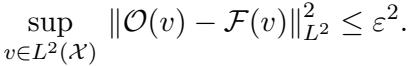
Our goal is to build an estimator \(\widehat{\mathcal{F}}_n\) using \(n\) training pairs \(\{(f_j, u_j)\}_{j=1}^n\) such that it approximates the true operator \(\mathcal{F}\) well. “Well” usually means minimizing the error in the \(L^2\) norm (the standard mean squared error for functions).

The Passive Trap

In the standard “passive” setting, we assume the input functions \(f\) are drawn randomly from some probability distribution \(\mu\). We train our model, and then we test it on new functions drawn from that same distribution.

The error we are trying to minimize looks like this:

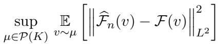
Here is the problem identified by the researchers: under standard assumptions in passive learning, the error convergence rate is often stuck at \(\approx n^{-1}\). That means to halve your error, you might need double the data. When data comes from expensive numerical solvers, that is a steep price to pay.

The Secret Weapon: Covariance Kernels

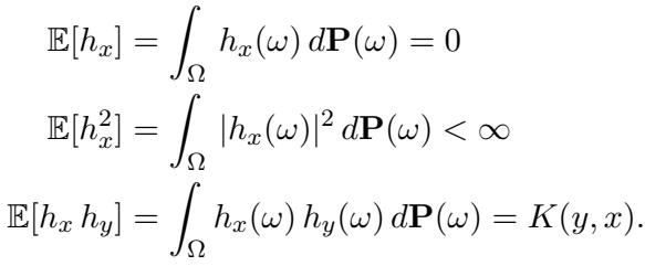
To do better than random sampling, we need to understand the structure of our input data. The authors assume the input functions are drawn from a stochastic process with a continuous covariance kernel \(K\).

If you are familiar with Gaussian Processes, this will ring a bell. The kernel \(K(x, y)\) describes the correlation between the function values at points \(x\) and \(y\). It essentially defines the “texture” or “smoothness” of the functions we expect to see.

Eigenvalues and Eigenfunctions

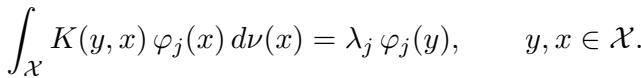
This is where the linear algebra magic happens. Any continuous kernel \(K\) can be decomposed using its eigenpairs \((\lambda_j, \varphi_j)\).

Think of these eigenfunctions \(\varphi_j\) as the “building blocks” or “basis functions” of the data distribution, and the eigenvalues \(\lambda_j\) as the “importance weights” of those blocks.

• \(\varphi_1\) is the most dominant shape in the data.
• \(\varphi_2\) is the second most dominant, and so on.
• The eigenvalues typically decay: \(\lambda_1 \ge \lambda_2 \ge \dots \ge 0\).

Mathematically, they satisfy this integral equation:

Because these inputs come from a stochastic process defined by \(K\), we can express any random input function \(v\) using the Karhunen-Loève (KL) Expansion. This is like a Fourier series, but tailored specifically to the probability distribution of our data:

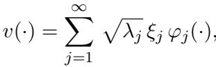
Here, \(\xi_j\) are uncorrelated random variables. This formula tells us that any input function is just a weighted sum of the eigenfunctions.

The Active Strategy: Don’t Guess, Query!

In Active Learning, the learner isn’t forced to accept random data. It can construct a specific input \(v\) and ask an “Oracle” (the PDE solver) for the corresponding output.

If you knew that your data was built entirely out of the blocks \(\varphi_1, \varphi_2, \dots\), what would you ask the Oracle?

You wouldn’t ask for a random messy combination. You would ask for the blocks themselves.

The Algorithm

The authors propose a deterministic strategy:

1. Identify the kernel \(K\) (which implies we know the distribution of inputs).
2. Compute the eigenfunctions \(\varphi_1, \dots, \varphi_n\) corresponding to the largest eigenvalues.
3. Query the Oracle using these eigenfunctions as inputs. We get outputs \(w_i = \mathcal{O}(\varphi_i)\).
4. Construct the Estimator:

The estimator is a linear operator built directly from these pairs:

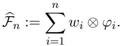
This looks like a tensor product. Effectively, this operator says: “If I see a function that looks like \(\varphi_i\), I will output \(w_i\).” Since any function in our distribution is a sum of \(\varphi_i\)’s, this estimator knows exactly how to handle the most important components of the data.

The Oracle isn’t Perfect

Real-world PDE solvers aren’t perfect. They have discretization errors (grid size) or numerical tolerances. The authors account for this by assuming the Oracle is an \(\varepsilon\)-approximate oracle.

This \(\varepsilon\) represents the “irreducible error”—the noise floor of our training data.

Theoretical Breakthrough: Arbitrarily Fast Convergence

The main contribution of the paper is proving that this active strategy is vastly superior to passive learning.

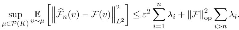
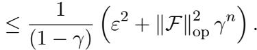
Theorem 1 (The Upper Bound) states that the error of the active estimator is bounded by two terms:

Let’s break this down:

1. The Irreducible Error (Left Term): \(\varepsilon^2 \sum_{i=1}^n \lambda_i\). This depends on the quality of your PDE solver (\(\varepsilon\)). If your solver is perfect (\(\varepsilon=0\)), this term vanishes.
2. The Reducible Error (Right Term): \(\|\mathcal{F}\|_{\mathrm{op}}^2 \sum_{i=n+1}^\infty \lambda_i\). This is the error due to stopping after \(n\) samples. It depends on the tail sum of the eigenvalues.

Why is this huge? In passive learning, you are stuck with a convergence rate of roughly \(n^{-1}\) regardless of how smooth your data is. In this active setting, the convergence rate depends on how fast the eigenvalues \(\lambda_i\) decay.

• If the eigenvalues decay exponentially, the error decays exponentially.
• If the eigenvalues decay polynomially (\(n^{-k}\)), the error follows suit.

We can achieve arbitrarily fast rates simply by having a kernel with fast-decaying eigenvalues.

Examples of Convergence

The authors provide specific examples to illustrate this:

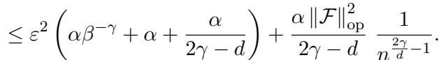
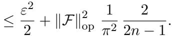
1. Shifted Laplacian Kernel: Common in PDE literature, this kernel yields polynomial decay. With specific parameters, the reducible error decays as:

2. RBF Kernel (Gaussian): The Radial Basis Function kernel is incredibly smooth. Its eigenvalues decay exponentially. Consequently, the active learning error vanishes exponentially:

3. Brownian Motion: Even for rougher processes like Brownian motion, the error decays nicely:

The Limitation of Passive Learning

You might ask, “Can’t I just get lucky with passive learning?”

The authors prove that the answer is no. Theorem 2 establishes a lower bound for any passive data collection strategy.

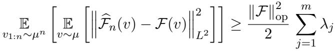
Even with a perfect oracle (\(\varepsilon=0\)) and infinite samples, passive learning is fundamentally limited by the variance of the estimation. The paper constructs a specific “hard” distribution where passive learners fail to converge efficiently, proving that the gap between active and passive methods is theoretical, not just experimental.

Experimental Evidence

Theory is great, but does it work in practice? The researchers tested their Active Linear Estimator against:

1. Passive Linear Estimator: The same math, but trained on random inputs.
2. Fourier Neural Operator (FNO): A state-of-the-art deep learning model for PDEs, trained on passive data.

They ran experiments on two classic problems: the Poisson Equation and the Heat Equation.

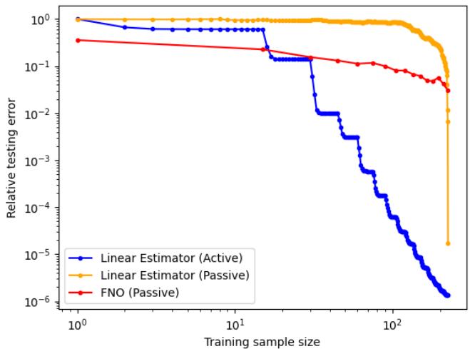
Poisson Equation Results

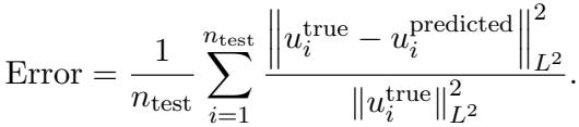
The setup involved solving \(-\nabla^2 u = f\) on a 2D grid.

The error metric used was the relative \(L^2\) error:

The Results: Look at the graph below. The Blue curve (Active Linear) drops like a stone. The Orange (Passive Linear) and Red (FNO Passive) struggle to keep up.

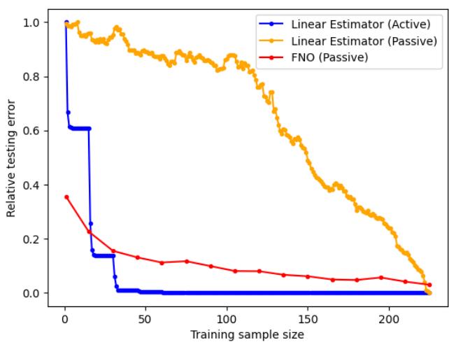
When viewed on a log-log scale, the difference is stark. The Active Linear Estimator achieves errors orders of magnitude lower than the passive methods with the same number of training samples (\(N\)).

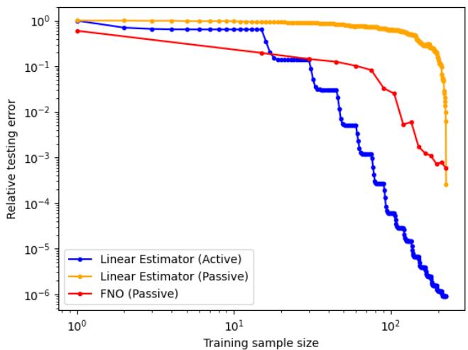
Heat Equation Results

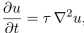
Similar results were found for the Heat equation, which involves time evolution.

Again, on the log scale, the Active Linear estimator (Blue) outperforms the passive variants significantly.

What about FNO with Active Data?

An interesting side note from the experiments (shown in the appendix of the paper) is that simply feeding active data to a Deep Learning model like FNO doesn’t automatically fix things. FNO is designed to generalize from i.i.d. samples. When fed the highly structured, non-i.i.d. eigenfunctions, it actually performed worse initially because the training distribution didn’t match the test distribution.

This highlights that active learning requires matching the estimator to the strategy. The Linear Estimator worked because it was mathematically designed to exploit the orthogonal nature of the eigenfunctions.

Conclusion and Key Takeaways

This research provides a rigorous mathematical foundation for something intuitive: Information matters more than volume.

By analyzing the covariance structure of the data (the Kernel), we can identify the “principal components” of the function space (the Eigenfunctions). Querying the simulator for these specific components allows us to reconstruct the solution operator with drastically fewer samples than random guessing.

Key Takeaways for Students & Practitioners:

1. Data Efficiency: If your simulation is expensive, do not just sample randomly. Look for active strategies.
2. Know Your Kernel: The smoothness and structure of your input data determine the theoretical limit of how fast you can learn.
3. Linearity is Powerful: For linear PDEs, simple linear estimators combined with smart data collection can outperform complex neural networks trained on “dumb” data.
4. The “Passive Barrier”: There is a hard limit to how fast you can learn from random samples (\(\sim n^{-1}\)). Active learning is the key to breaking that barrier.

As we move toward digital twins and real-time physics simulations, techniques like this—which squeeze the maximum information out of every expensive computation—will become the new standard.