The capabilities of Large Language Models (LLMs) have exploded in recent years, particularly regarding context length. We have moved from models that could barely remember a paragraph to beasts like Llama-3-1M and Gemini-1.5 that can digest entire novels, codebases, or legal archives in a single pass.

However, this capability comes with a massive computational cost. As the context length grows, so does the memory required to store the Key-Value (KV) cache—the stored activations of previous tokens used to generate the next one. For a 1-million-token sequence, the KV cache can easily exceed the memory capacity of even top-tier GPUs like the Nvidia A100.

This creates a dilemma: do we drop information to save memory (risking accuracy), or do we offload data to the CPU (killing inference speed due to slow transfer rates)?

In this post, we will dive deep into ShadowKV, a new research paper that proposes a clever third option. By understanding the mathematical properties of the KV cache, the authors developed a system that keeps “shadow” representations on the GPU while offloading the bulk of the data to the CPU, achieving up to 6x larger batch sizes and 3x higher throughput without sacrificing accuracy.

The Problem: The KV Cache Bottleneck

To understand why ShadowKV is necessary, we first need to understand the bottleneck in modern LLM inference.

When an LLM generates text, it is autoregressive—it predicts the next token based on all previous tokens. To avoid recalculating the entire history for every new word, we save the Key and Value matrices of the attention mechanism in GPU memory. This is the KV Cache.

As context length (\(S\)) increases, the KV cache grows linearly. For long-context models (e.g., 100k+ tokens), this cache becomes massive.

1. Memory Wall: You run out of high-bandwidth GPU memory (HBM). This forces you to reduce the batch size (the number of requests processed simultaneously), which hurts throughput.
2. Bandwidth Wall: Even if you have the memory, moving that much data from memory to the compute units for every token generation takes time.

Existing Solutions and Their Flaws

Researchers have tried several tricks to mitigate this, but most have significant downsides:

• Token Eviction: This method simply deletes “unimportant” tokens from the cache. While fast, it often leads to information loss, causing the model to forget earlier context or fail at tasks requiring high precision (like coding).
• Sparse Attention (GPU-resident): These methods keep all data on the GPU but only compute attention on a subset. This speeds up math but doesn’t solve the memory capacity issue.
• CPU Offloading: This approach moves the KV cache to the CPU’s RAM (which is cheap and plentiful) and fetches only what is needed. The problem? The PCIe bus connecting the CPU and GPU is slow. Fetching data introduces massive latency.

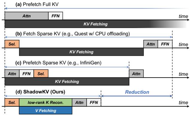
Figure 4 below illustrates how ShadowKV compares to these methods. Note how traditional offloading (Graph b) and prefetching (Graph c) still struggle with latency or complexity. ShadowKV (Graph d) introduces a unique pipeline that reconstructs low-rank keys on the fly.

The Core Insights

The ShadowKV team didn’t just engineer a faster pipeline; they analyzed the mathematical structure of the KV cache and found two crucial properties that make their method possible.

Insight 1: Pre-RoPE Keys are Low-Rank

LLMs typically use Rotary Positional Embeddings (RoPE) to encode the position of tokens. The researchers performed Singular Value Decomposition (SVD) on the weights and caches of Llama-3 models.

They discovered something fascinating: The Key (K) cache is extremely low-rank before RoPE is applied.

In linear algebra, a “low-rank” matrix contains a lot of redundant information and can be compressed significantly without losing much data. However, once RoPE is applied, the rotation makes the matrix “full rank” and hard to compress. Furthermore, the Value (V) cache is never low-rank; it is dense with information.

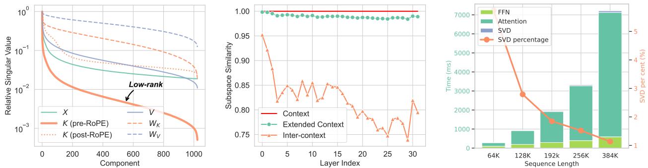
As shown in the left chart of Figure 1, the “Pre-RoPE Key” (the green line) drops off sharply in singular values, indicating it is highly compressible (low-rank). The Value cache (purple line) stays high, meaning it cannot be easily compressed.

The Strategy: We can compress the Key cache by storing only its low-rank projection on the GPU. The bulky Value cache must be moved to the CPU, but since we only need to fetch specific parts of it, that might be manageable.

Insight 2: Values Need to be Offloaded, Keys Can be Reconstructed

Since the Value cache takes up half the memory but isn’t compressible, ShadowKV offloads it entirely to the CPU. The Key cache, however, is kept on the GPU—but in a highly compressed, low-rank form.

During inference, ShadowKV reconstructs the full Key cache from the compressed version on the fly inside the GPU. This is computationally cheap compared to the cost of moving data over the PCIe bus.

Insight 3: Accurate Sparse Selection via Landmarks

To avoid computing attention over the entire 1-million-token context, we need Sparse Attention. We only want to attend to the most relevant tokens.

But how do we know which tokens are relevant without loading them first?

The researchers found that tokens usually exhibit “spatial locality.” If a token is relevant, its neighbors are likely relevant too. Therefore, they group tokens into chunks (e.g., size 8). They calculate the average (mean) of the Key cache for that chunk and store it as a “Landmark”.

By comparing the current query against these Landmarks, the model can predict which chunks are important. It then only fetches the Value data for those specific chunks from the CPU.

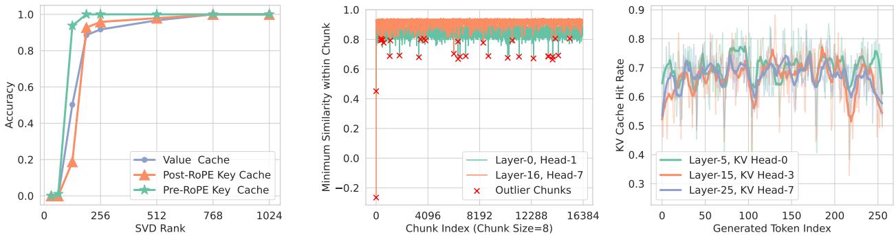
Figure 5 (Middle) shows that while most chunks can be approximated by their mean (high similarity), there are a few Outliers (the red crosses). These are chunks that are mathematically distinct and difficult to approximate. ShadowKV detects these rare outliers during the pre-filling phase and keeps them permanently in the GPU’s high-speed memory to ensure accuracy doesn’t drop.

The ShadowKV Method

Combining these insights, the authors propose a system that splits the workload between GPU and CPU.

The Architecture

As illustrated in Figure 3, the system operates in two phases:

1. Pre-filling (Left):

• The model processes the input prompt.
• Keys: It takes the Pre-RoPE Keys and compresses them using SVD. These small, low-rank keys stay on the GPU.
• Landmarks: It groups keys into chunks and calculates the mean (Landmark) for each. These stay on the GPU.
• Outliers: It identifies the few chunks that don’t fit the approximation and keeps them on the GPU.
• Values: The heavy Value cache is sent to the system RAM (CPU).

2. Decoding (Right):

• When generating a new token, the model uses the Landmarks to score which chunks are relevant to the current query.
• Parallel Execution: This is the magic step. The system simultaneously:
• Fetches Values: Requests only the top-k relevant Value chunks from the CPU.
• Reconstructs Keys: Uses the low-rank projections on the GPU to rebuild the relevant Key chunks and applies RoPE.
• Because the Value fetching (memory bound) and Key reconstruction (compute bound) happen at the same time, the latency of fetching data is effectively hidden.

Theoretical Bandwidth

Why goes through all this trouble? It comes down to Equivalent Bandwidth. By reducing the amount of data transferred and compressing the data that stays, ShadowKV simulates a GPU with much higher memory bandwidth than actually exists.

\[ { \widetilde { B } } = \frac { 2 S B _ { \mathrm { G P U } } } { S / C + 2 ( K + O ) C + ( 1 - \alpha ) K C B _ { \mathrm { G P U } } / B _ { \mathrm { P C I e } } } \]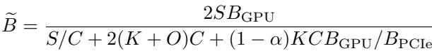

The equation above calculates this “equivalent bandwidth.” Don’t worry about the complex variables; the takeaway is visually represented in Figure 2 below.

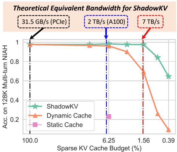
The chart shows that ShadowKV (green star line) maintains high accuracy even when the “Sparse KV Cache Budget” (the amount of data actively used) is very low. Theoretically, on an A100 GPU, ShadowKV can achieve an equivalent bandwidth of 7 TB/s—far exceeding the physical hardware limit of 2 TB/s.

Experimental Results

Does this complex architecture actually deliver on its promises? The authors tested ShadowKV on major benchmarks including RULER, LongBench, and “Needle In A Haystack.”

Accuracy Maintenance

The biggest risk with sparse attention and compression is that the model gets “stupid”—it forgets details hidden in the long context.

Table 1 compares ShadowKV against other methods like Quest, InfiniGen, and Loki.

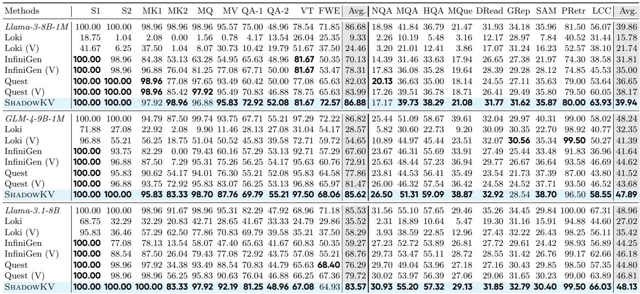
The results are impressive. ShadowKV (highlighted in bold rows) consistently matches the accuracy of the original model (“Full Attention”), even on tasks requiring precise retrieval like “Variable Tracking” (VT) or Question Answering (QA). Competing methods often see accuracy plummet (e.g., Loki scores drop to near zero on some tasks).

Visualizing Retrieval: Needle In A Haystack

The “Needle In A Haystack” test hides a specific fact (the needle) somewhere in a massive block of text (the haystack) and asks the model to find it.

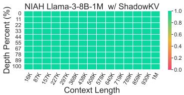
Figure 6 shows the results for Llama-3-8B-1M. The entire heatmap is green, meaning ShadowKV successfully retrieved the information regardless of where it was located in the context (from 1K up to 1M tokens) or the depth of the document.

Multi-Turn Conversations

A common failure mode for eviction-based strategies (like SnapKV or StreamingLLM) is multi-turn chat. If you delete “unimportant” tokens during the first question, you might realize they are crucial for the second question—but they are gone forever.

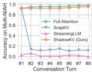
Figure 7 demonstrates this clearly. While SnapKV (blue line) crashes after the first turn, ShadowKV (orange line) maintains near-perfect accuracy across 8 turns of conversation, behaving almost identically to Full Attention (green line).

Throughput and Efficiency

Finally, let’s look at speed. The primary goal was to increase throughput and batch size.

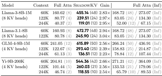
Table 3 shows the throughput on an Nvidia A100 GPU.

• Llama-3-8B-1M (122K context): Standard Full Attention achieves 80 tokens/s with a batch size of 4. ShadowKV achieves 239 tokens/s with a batch size of 24.
• Infinite Batch Assumption: The rightmost column shows that ShadowKV is so efficient that it sometimes outperforms the theoretical maximum speed of Full Attention assuming infinite GPU memory.

By offloading the heavy Value cache to the CPU, ShadowKV frees up massive amounts of GPU memory. This allows you to run 6x larger batch sizes (e.g., batch size 48 vs 8 for 60K context), which is the most effective way to saturate GPU compute and maximize throughput.

Conclusion

The “Memory Wall” has long been the enemy of long-context LLM deployment. ShadowKV offers a compelling solution that refuses to compromise. It doesn’t blindly delete data (like eviction methods), nor does it let the CPU bus stall the GPU (like naive offloading).

By recognizing that Keys are compressible and Values are offloadable, ShadowKV orchestrates a symphony of low-rank reconstruction and sparse fetching. It effectively creates a “shadow” cache that allows standard GPUs to punch far above their weight class, handling 1-million-token contexts with the speed and accuracy of much smaller sequences.

For students and practitioners, this paper highlights a vital lesson: hardware constraints (like GPU memory) are often best solved not just by buying more hardware, but by understanding the underlying mathematical structure of the data you are processing.

---