The Stylistic Fingerprint: Solving Authorship Attribution with Bayesian LLMs

Imagine finding a lost manuscript claiming to be a forgotten work by Jane Austen or identifying the anonymous creator behind a coordinated misinformation campaign on social media. These scenarios rely on authorship attribution—the computational science of determining who wrote a specific text based on linguistic patterns.

For decades, this field relied on manually counting words or, more recently, fine-tuning heavy neural networks. But a new paper, A Bayesian Approach to Harnessing the Power of LLMs in Authorship Attribution, proposes a fascinating shift. Instead of training models to classify authors, the researchers leverage the raw, pre-trained probabilistic nature of Large Language Models (LLMs) like Llama-3.

In this post, we will dissect how this method works, why it outperforms traditional techniques in “one-shot” scenarios, and how it turns the generative power of LLMs into a precise forensic tool.

The Problem: Identifying the Ghost in the Machine

Authorship attribution is the digital equivalent of handwriting analysis. Every author has a unique “stylometric” fingerprint—a combination of vocabulary, sentence structure, punctuation habits, and grammatical idiosyncrasies.

Historically, solving this problem involved two main approaches:

1. Stylometry: Statistical methods that count features (like how often someone uses the word “the” or “however”). These are interpretable but often miss complex, long-range dependencies in text.
2. Fine-tuned Neural Networks: taking a model like BERT and retraining it specifically on a dataset of authors. While accurate, this is computationally expensive, data-hungry, and requires retraining the model every time a new author is added to the suspect list.

Enter Large Language Models

With the rise of GPT-4 and Llama-3, we have models that have “read” nearly the entire internet. They understand style implicitly. However, simply asking an LLM, “Who wrote this text?” (a technique called Question Answering or QA) yields poor results. LLMs are prone to hallucinations and often struggle to choose correctly from a long list of potential candidates.

The researchers behind this paper argue that we are using LLMs wrong. Instead of treating them as chatbots that generate answers, we should treat them as probabilistic engines that score likelihoods.

The Core Method: A Bayesian Approach

The heart of this paper is a method coined the LogProb approach. It combines classical Bayesian statistics with the modern architecture of Transformers.

1. The Bayesian Framework

The goal is simple: Given an unknown text \(u\) and a set of candidate authors, we want to find the probability that a specific author \(a_i\) wrote \(u\).

Mathematically, this is expressed using Bayes’ Theorem:

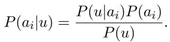
Here:

• \(P(a_i|u)\) is the posterior: the probability the author wrote the text.
• \(P(u|a_i)\) is the likelihood: the probability of the text existing, assuming that specific author wrote it.
• \(P(a_i)\) is the prior: how likely the author is to be the writer before we see the text (usually assumed equal for all candidates).

Since \(P(u)\) (the probability of the text occurring generally) is constant across all authors, the task boils down to calculating the likelihood \(P(u|a_i)\). If we can accurately measure how likely it is that Author A produced Text U, we can solve the mystery.

2. From Authors to Textual Entailment

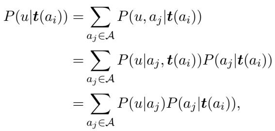
To calculate \(P(u|a_i)\), the researchers use a set of known texts provided by the author, denoted as \(t(a_i)\). They rely on the assumption that if an author wrote the known texts, the “style” distribution of the unknown text \(u\) should match.

Through a series of derivations relying on the assumption that texts from the same author are independent and identically distributed (i.i.d.), the researchers expand the probability calculation:

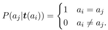
This looks complex, but it simplifies significantly under the “sufficient training set” assumption. Ideally, the known texts \(t(a_i)\) are distinctive enough that they could only come from author \(a_i\). This turns the probability of other authors producing those exact known texts to zero:

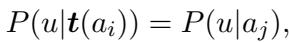
This leads to a clean, usable equality where the probability of the unknown text given the known texts is effectively the probability of the text given the author:

3. Using the LLM as a Probability Calculator

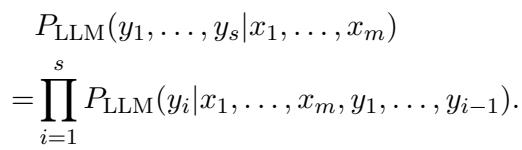
This is where the Large Language Model comes in. LLMs are autoregressive—they predict the next token based on previous tokens. When an LLM generates text, it calculates probabilities for every possible next word in its vocabulary.

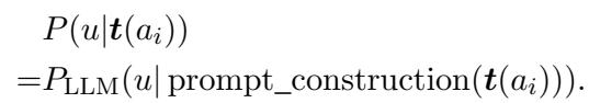
The researchers use this to measure entailment. They construct a prompt that includes the known text from an author, and then append the unknown text. They don’t ask the LLM to generate text; they force-feed the unknown text into the model and ask, “How surprised are you by this sequence of words?”

If the LLM has seen the author’s writing style in the prompt, and the unknown text matches that style, the LLM will assign a high probability to the tokens in the unknown text.

The probability of a sequence of tokens (\(y_1\) to \(y_s\)) given a context (\(x_1\) to \(x_m\)) is the product of the probabilities of each individual token:

4. The Algorithm in Action

The “LogProb” method puts it all together. To check if an unknown text \(u\) belongs to a known author, the system:

1. Takes the known texts from the author (\(t(a_i)\)).
2. Constructs a prompt (e.g., “Here is a text from the same author:”).
3. Feeds this into the LLM.
4. Calculates the probability of the unknown text \(u\) following that prompt.

The system repeats this process for every candidate author. The candidate that results in the highest probability (or least “surprise”) is identified as the author.

The overall architecture is visualized below. Note how the unknown text is evaluated against every candidate author’s model instance to find the best fit.

Experiments and Results

To test this theory, the researchers used two datasets: IMDb62 (movie reviews from 62 prolific users) and a Blog dataset (posts from thousands of bloggers).

They set up a “one-shot” learning scenario: the model only gets one known article from a candidate to learn their style before trying to attribute a new anonymous text.

Comparison with Baselines

The results were impressive. The researchers compared their LogProb method using Llama-3-70B against:

• QA Methods: Asking GPT-4 or Llama-3 “Who wrote this?”
• Embedding Methods: BERT-based models (BertAA, GAN-BERT) that require training.

The LogProb method achieved roughly 85% accuracy on the IMDb dataset with 10 candidates.

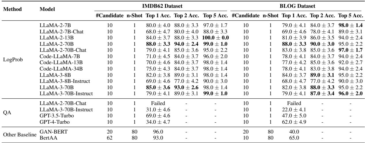
Key Takeaways from the Results:

1. QA Fails: As seen in the table (labeled QA), asking models directly results in poor performance (34% for GPT-4-Turbo). The models struggle to reason explicitly about authorship.
2. LogProb Succeeds: The Bayesian approach with Llama-3-70B hits 85% accuracy, rivaling or beating methods that require extensive fine-tuning.
3. No Training Required: Unlike GAN-BERT, which needs to be retrained for every new set of authors, the LogProb method works instantly with just a prompt.

The Challenge of Scale

A common issue in authorship attribution is that accuracy plummets as you add more suspects. If you have 50 potential authors, it’s much harder to pick the right one than if you have 2.

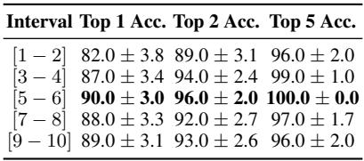
The researchers analyzed how the LogProb method scales.

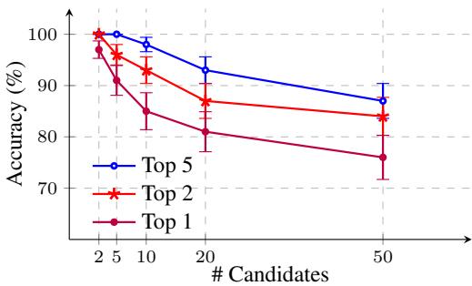
As shown above, while the “Top 1” accuracy (finding the exact author) drops as the candidate pool grows to 50, the Top 5 accuracy remains robust (nearly 90%). This means even if the model doesn’t pick the exact author first, the correct author is almost always in the top few suggestions. This is incredibly valuable for forensic teams narrowing down a suspect list.

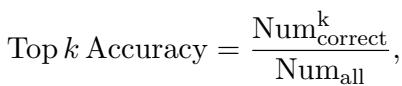
For reference, the “Top k Accuracy” metric is defined as:

Sensitivity to Prompts

Does the specific wording of the prompt matter? If we say “Analyze the writing style” versus just “Here is text,” does the accuracy change?

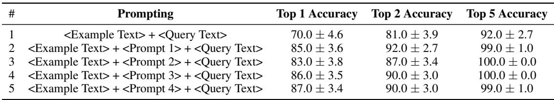
The study found that using some prompt is better than none (Row 1 vs Rows 2-5). However, the specific phrasing of the prompt (Prompt 1 vs Prompt 4) had very little impact on the final score. This suggests the method is robust and doesn’t require fragile “prompt engineering” to work.

Bias and Subgroup Analysis

An interesting, perhaps sociolinguistic, finding emerged regarding gender and age.

Gender Differences

The model found it easier to attribute authorship to female bloggers than male bloggers.

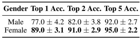
As shown in the table above, the Top-1 accuracy for female authors (89.0%) was significantly higher than for male authors (77.0%). The authors hypothesize that the female-authored blogs in this dataset may contain more distinct personal stylistic markers, making them easier to fingerprint.

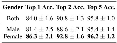
We can see the aggregate gender data here as well:

Age and Content Rating

The researchers also looked at the age of the authors and the content of the reviews.

• Age: Younger authors (13-17) were much easier to identify (90% accuracy) compared to older authors (33-40, roughly 88%). This aligns with linguistic theories that younger demographics often use more distinctive, evolving slang and stylistic choices.
• Ratings: In the IMDb dataset, extreme reviews (very high or low ratings) were slightly harder to attribute than middle-of-the-road reviews (ratings 5-6), which achieved the highest accuracy.

Efficiency: Speed vs. Cost

Finally, why use this method over standard Question Answering? Aside from accuracy, there is a massive efficiency argument.

In a QA approach, the LLM has to generate tokens one by one to write out the author’s name. In the LogProb approach, the model only performs a single forward pass to calculate probabilities.

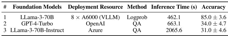
As the table shows, the LogProb method is drastically faster (462 seconds vs 2065 seconds) while being far more accurate.

Conclusion

The paper A Bayesian Approach to Harnessing the Power of LLMs in Authorship Attribution marks a significant step forward in forensic linguistics. By treating Large Language Models not as creative writers but as probabilistic calculators, the authors unlocked a powerful, training-free method for identifying authorship.

This “LogProb” method:

1. Removes the need for fine-tuning, saving computational resources.
2. Outperforms direct questioning of LLMs by a massive margin.
3. Scales well across many candidates and handles limited data (one-shot) effectively.

While limitations exist—such as the high cost of running 70B parameter models and the potential biases inherited from training data—this research demonstrates that the true power of LLMs might lie beneath the surface of their generated text, deep in the mathematical probabilities that drive them. For students and researchers in NLP, this is a compelling reminder that sometimes the best way to use a model is to stop asking it questions and start measuring its surprise.