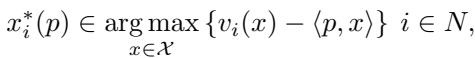
](https://deep-paper.org/en/paper/2411.09355/images/cover.png)
Allocating resources efficiently is one of the fundamental problems in economics. When the resources are simple—like shares of a company—standard markets work well. But what happens when the items are distinct, but their values are interconnected?
Consider a government auctioning spectrum licenses to telecom companies. A license for New York City is valuable, and a license for Philadelphia is valuable. But to a telecom provider, having both might be worth significantly more than the sum of the parts because it allows them to build a continuous network. Conversely, two different frequencies in the same city might be substitutes.
This is the domain of Combinatorial Auctions (CAs). The challenge? The number of possible bundles grows exponentially with the number of items. If there are 100 items, there are \(2^{100}\) possible bundles—far too many for any bidder to list values for.
To solve this, researchers have turned to Iterative Combinatorial Auctions (ICAs), where the auctioneer and bidders interact over rounds. Recently, Machine Learning (ML) has entered the fray to make these auctions smarter. However, a major rift has existed between two approaches: asking about Prices (easier for humans, less efficient) vs. asking about Values (efficient, but cognitively exhausting).
In this post, we explore a new framework, the Machine Learning-powered Hybrid Combinatorial Auction (MLHCA). This mechanism unifies these two paradigms, using ML to blend “Price” and “Value” queries. It achieves state-of-the-art efficiency while respecting the cognitive limits of human bidders.
The Core Tension: Demand vs. Value
Before understanding the solution, we have to understand the specific tools an auctioneer can use to extract information from bidders.
1. The Demand Query (DQ)
This is the standard market interaction. The auctioneer sets a price tag for every item. The bidder looks at the prices and says, “At these prices, I want this bundle.”
Mathematically, the bidder \(i\) sees a price vector \(p\) and chooses the bundle \(x\) that maximizes their surplus (value minus cost):
- Pros: This is natural. It’s how we shop at a supermarket. It lowers cognitive load because the bidder only has to solve a maximization problem for the current prices.
- Cons: It provides “low-resolution” information. If you buy an apple for \(1, the auctioneer knows you value the apple at at least \)1, but not whether you value it at \(1.01 or \)100.
2. The Value Query (VQ)
Here, the auctioneer presents a specific bundle \(x\) and asks, “Exactly how much is this bundle worth to you?”
- Pros: High precision. It gives the auctioneer exact data points on the valuation function.
- Cons: Cognitive overload. Imagine being asked, “What is your exact dollar value for a bundle containing Spectrum A, Spectrum C, and Spectrum F?” without any price context. It is incredibly difficult for humans to estimate absolute values for random bundles in a vacuum.
The Status Quo
Practical auctions (like the famous Combinatorial Clock Auction or CCA) use Demand Queries because they are practical. Recent academic work (like BOCA) uses Value Queries driven by ML because they are theoretically efficient, but they struggle in the real world because bidders can’t answer random value questions effectively.
The Learning Problem
In an ML-powered auction, the goal is to train a model (specifically a Neural Network) to learn each bidder’s private valuation function \(v_i(x)\). The auctioneer uses this model to predict which bundles are efficient to allocate.
The researchers behind MLHCA identified a critical flaw in relying on just one type of query.
The Flaw of Value Queries (VQs): If you start an auction with VQs, you are essentially shooting in the dark. In a high-dimensional space, the probability of randomly asking about a “good” bundle (one the bidder actually wants) is near zero. ML models trained on random VQs fail to capture the “high-value” regions of the space.
The Flaw of Demand Queries (DQs): DQs are great at finding the “high-value” regions because bidders naturally select good bundles. However, they fail to pin down the exact value. As proved in the paper, a DQ-based auction cannot guarantee full efficiency, even with infinite queries.
To bridge this gap, the researchers propose Mixed Query Learning. They initialize the auction with Demand Queries to find the relevant parts of the bundle space, and then switch to Value Queries to pin down the exact numbers.
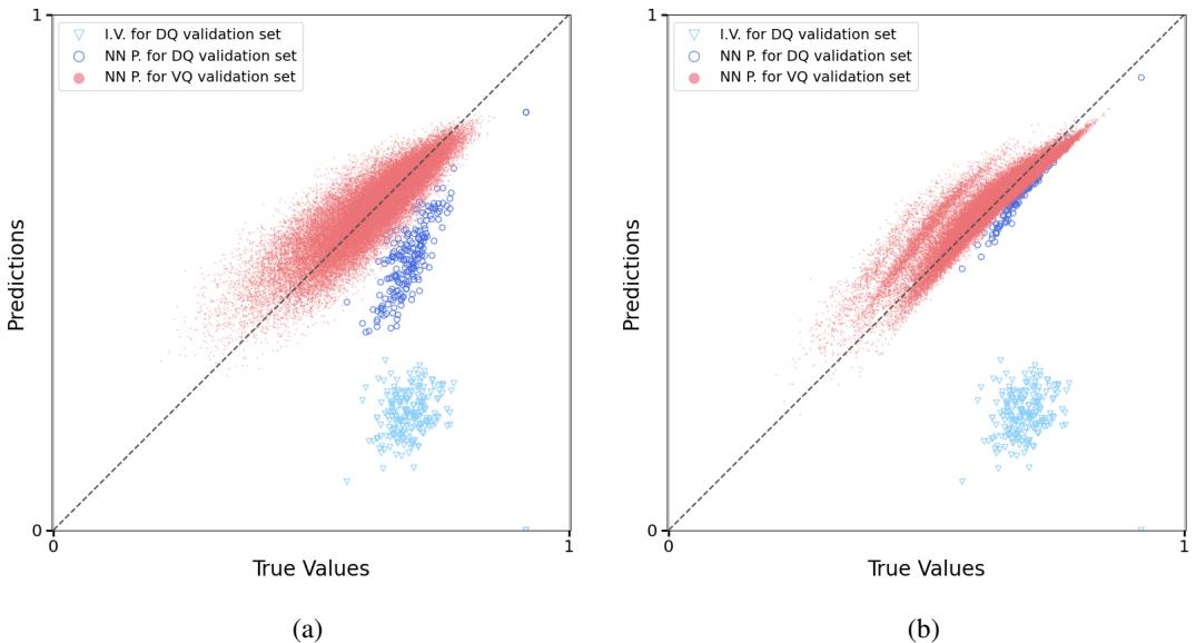
Visualizing the Learning Benefit
The image below shows the performance of a Neural Network predicting a bidder’s values.
- Plot (a) shows a model trained only on Demand Queries. Notice the blue dots (predictions for bundles the bidder actually wants). They form a line parallel to the truth, but shifted. The model learned the structure of preferences (relative value) but not the magnitude (absolute value).
- Plot (b) shows the Mixed model. By adding Value Queries, the model “snaps” to the diagonal. It knows both the structure and the absolute numbers.
The Mechanism: MLHCA
The MLHCA is designed as a phased process. It transitions from coarse exploration (prices) to precise exploitation (values).
Here is the high-level workflow of the auction:

Phase 1: The Combinatorial Clock (Lines 3-6)
The auction starts like a standard Combinatorial Clock Auction (CCA). Prices start low and rise on items with excess demand. This serves as a “warm-up,” generating easy initial data points (DQs) where bidders reveal their general interests.
Phase 2: ML-Powered Demand Queries (Lines 7-12)
Once the initial phase is done, the ML engine turns on. The auctioneer trains a Monotone-Value Neural Network (mMVNN) on the data collected so far.
Instead of just raising prices by a fixed percentage, the auctioneer uses the ML model to generate “Smart Prices.” They solve an optimization problem to find price vectors that are most likely to clear the market (match supply and demand) based on what the model knows about the bidders.
Phase 3: The “Bridge Bid” (Lines 17-18)
This is a theoretically critical innovation. The transition from Demand Queries (prices) to Value Queries (direct questions) can actually be dangerous. The researchers prove that naively switching query types can cause a sudden drop in efficiency (regret).
To prevent this, they introduce the Bridge Bid. Before starting the Value Query phase, the auctioneer asks one specific question:
“What is your exact value for the bundle you are currently holding (in the inferred allocation)?”
This single data point anchors the ML model, ensuring the efficiency of the auction can only go up, not down.
Phase 4: ML-Powered Value Queries (Lines 19-35)
Now that the ML model has a good “sketch” of the valuation landscape (from DQs) and is anchored correctly (from the Bridge Bid), it starts asking specific Value Queries. It uses the ML model to solve the Winner Determination Problem (WDP): finding the allocation that maximizes social welfare according to the model, and then querying the specific bundles involved in that allocation.
The Math Behind the Curtain
The “Inferred Value” is central to how the auctioneer makes decisions. Even if a bidder hasn’t stated their exact value for a bundle, their previous answers set a lower bound.
If a bidder sees prices \(p\) and picks bundle \(x\), we know their profit for \(x\) is higher than for any other bundle \(y\) (conceptually). This allows the auctioneer to construct a lower-bound function \(\tilde{v}_i\):
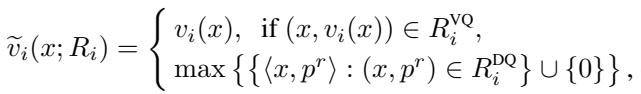
The first case is simple: if we asked a Value Query, we know the value \(v_i(x)\). The second case handles Demand Queries: the inferred value is the maximum lower bound consistent with the bidder’s previous price responses.
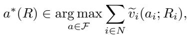
The auctioneer always computes the winner based on these inferred values:
Experimental Results
Does this hybrid approach actually work? The researchers tested MLHCA on the Spectrum Auction Test Suite (SATS), the gold standard for simulating large-scale spectrum auctions.
They compared MLHCA against:
- CCA: The standard non-ML auction used in the real world.
- ML-CCA: An ML auction using only prices (DQs).
- BOCA: The state-of-the-art ML auction using only values (VQs).
Efficiency and Convergence
The graph below plots “Efficiency Loss” (lower is better) against the number of bids/queries.
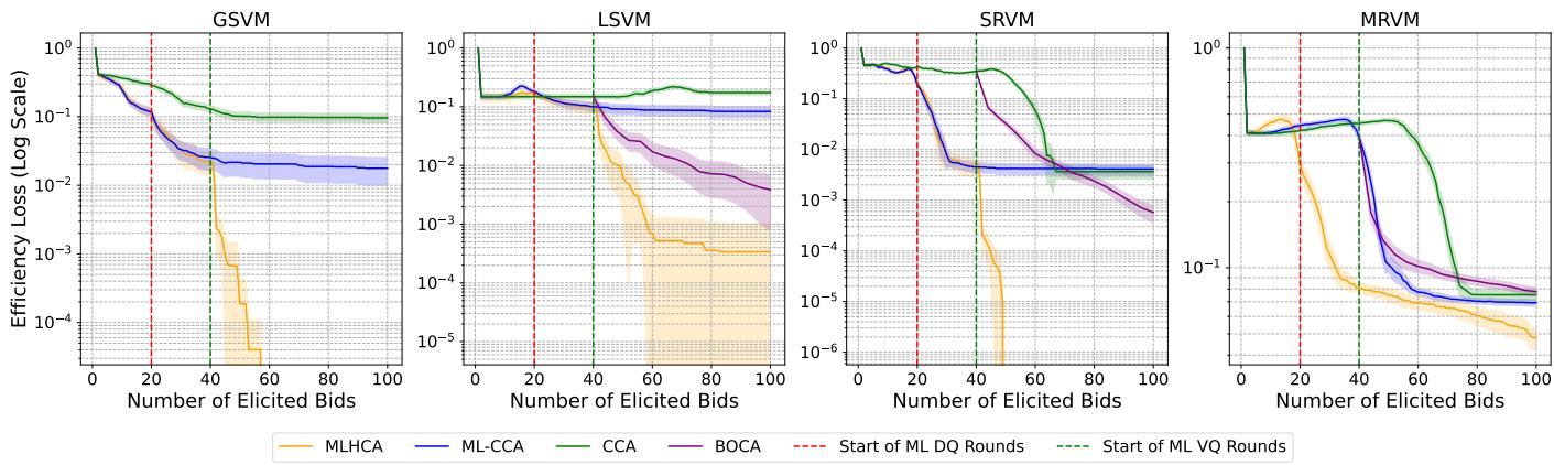
- Early Game (0-40 bids): MLHCA (Orange) matches ML-CCA (Blue). It uses prices, which are very effective early on. Notice how BOCA (Purple), which uses random VQs, struggles to improve efficiency initially—it’s “lost” in the high-dimensional space.
- Late Game (40+ bids): At bid 40, MLHCA switches to Value Queries (marked by the red dashed line). The efficiency loss plummets immediately. It outperforms ML-CCA (which gets stuck) and stays ahead of BOCA.
In the MRVM domain (Multi-Region Value Model), which most closely simulates realistic 4G spectrum auctions, MLHCA reduces efficiency loss by a factor of 10 compared to the previous state-of-the-art. In dollar terms, for a multi-billion dollar spectrum auction, this could represent hundreds of millions of dollars in gained social welfare.
The Importance of the Bridge Bid
The theory warned that switching query types could hurt efficiency. The experiments confirmed the solution. The plot below shows MLHCA with (orange) and without (blue) the Bridge Bid.
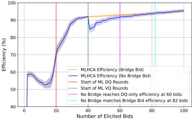
Without the Bridge Bid, efficiency actually drops when Value Queries start (around bid 40). It takes about 20 additional queries just to recover to the previous level. With the Bridge Bid, the transition is smooth and monotonic.
Conclusion
The MLHCA represents a maturation of Machine Learning in Mechanism Design. Rather than trying to force a purely “ML-native” approach (like doing only Value Queries), it respects the economic and human realities of auctions:
- Start with Prices (DQs): They are cognitively easy and great for “global exploration” of what bidders generally want.
- Finish with Values (VQs): They provide the mathematical precision needed for optimal allocation.
- Use ML as the Glue: The Neural Network integrates these two disparate data streams into a single coherent model of bidder preferences.
By strategically combining these query types, MLHCA establishes a new benchmark. It creates auctions that are not only mathematically more efficient but also faster to converge and easier for human participants to trust and use.