Introduction

In the world of decision-making, data is king. But data is also messy, finite, and noisy. Whether you are managing a stock portfolio, stocking inventory for a store, or training a machine learning model, you rarely know the true mechanism generating your data. Instead, you have to estimate it.

The standard approach is to gather data, fit a probability distribution (your model), and make the decision that minimizes your expected risk based on that model. In a Bayesian framework, you go a step further: you combine your data with prior beliefs to get a posterior distribution, giving you a better sense of parameter uncertainty.

But here is the catch: What if your estimated model—even the Bayesian one—is slightly wrong?

When you optimize aggressively against a single estimated model (or an average of them), you often fall victim to the Optimizer’s Curse. You tune your decision so perfectly to the specific quirks of your limited data that performance collapses when you face the real world. You are “overfitting” your decision to your uncertainty.

This post explores a fascinating solution presented in the paper Decision Making under the Exponential Family: Distributionally Robust Optimisation with Bayesian Ambiguity Sets. The authors introduce a framework called DRO-BAS. It combines the uncertainty quantification of Bayesian statistics with the safety net of Distributionally Robust Optimisation (DRO). The result is a method that is not only mathematically elegant but computationally faster and empirically safer than existing alternatives.

Background: The Decision Maker’s Dilemma

Before diving into the new method, let’s set the stage with the three main players in this story: The Standard Bayesian, The Robust Optimizer, and the “Existing” Hybrid.

1. The Standard Bayesian

In a standard Bayesian Risk Optimization (BRO), you look at your posterior distribution (your beliefs about the model parameters after seeing data) and minimize the expected loss.

\[ \operatorname* { m i n } _ { x \in \mathcal { X } } \mathbb { E } _ { \theta \sim \Pi ( \theta | \mathcal { D } ) } \left[ \mathbb { E } _ { \xi \sim \mathbb { P } _ { \theta } } [ f _ { x } ( \xi ) ] \right] . \]

While this accounts for parameter uncertainty, it assumes your Bayesian model is correct. If the real world (the Data Generating Process, or DGP) deviates from your model family or if your prior was misspecified, this approach offers no insurance.

2. The Robust Optimizer (DRO)

Distributionally Robust Optimisation (DRO) takes a worst-case view. Instead of optimizing for one distribution, you define an Ambiguity Set—a “ball” of distributions close to your estimate. You then find the decision that minimizes the worst possible risk inside that ball. If you are safe against the worst case in the ball, you are likely safe against the real world.

3. The Existing Hybrid (BDRO)

Previous attempts to combine these, like Bayesian DRO (BDRO), tried to average the robustness. They would sample parameters from the posterior, construct a small ambiguity ball around each one, calculate the worst-case risk for each, and then average those risks.

\[ ( B D R O ) \underset { x \in \mathcal { X } } { \mathrm { m i n } } \ \mathbb { E } _ { \theta \sim \Pi ( \theta | \mathcal { D } ) } \left[ \operatorname* { s u p } _ { \mathbb { Q } \in \mathcal { B } _ { \epsilon } ( \mathbb { P } _ { \theta } ) } \ \mathbb { E } _ { \xi \sim \mathbb { Q } } [ f _ { x } ( \xi ) ] \right] , \]

While better than nothing, BDRO is computationally heavy. It is a “two-stage” problem: you have to solve a maximization problem (finding the worst risk) inside an expectation integral. In practice, this requires a nested loop of sampling that is slow and inefficient. Furthermore, it doesn’t strictly correspond to a single “worst-case” distribution, making it harder to interpret.

The Solution: Bayesian Ambiguity Sets (DRO-BAS)

The researchers propose a cleaner, more rigorous approach: DRO-BAS. Instead of averaging the worst-case scenarios of many models, why not define a single ambiguity set that incorporates the Bayesian posterior directly?

They propose two specific ways to construct these sets, shown in the definitions below:

Let’s break these down visually and mathematically.

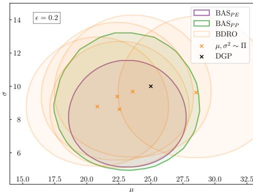
As shown in Figure 1 above, the approaches differ in geometry:

• BDRO (Existing): Takes the expectation of worst-case risks around individual posterior samples (the orange crosses).
• BAS-PP (Green): A ball centered around the posterior predictive distribution.
• BAS-PE (Purple): A set defined by the expected KL divergence from the model family.

1. BAS via Posterior Predictive (DRO-BAS\(_{PP}\))

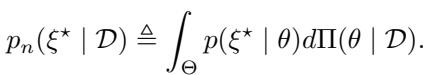
The most intuitive way to combine Bayesian inference with DRO is to look at the Posterior Predictive Distribution (\(\mathbb{P}_n\)). This is the single distribution you get when you average all your possible models weighted by their posterior probability.

The BAS\(_{PP}\) method simply creates a standard Kullback-Leibler (KL) divergence ball centered on this predictive distribution:

The objective is to minimize the worst-case risk within this ball:

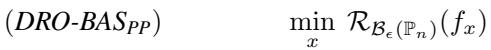
The Good: This is a pure “worst-case” approach. It admits a strong dual formulation, meaning we can convert the complex minimization-maximization problem into a simpler minimization problem:

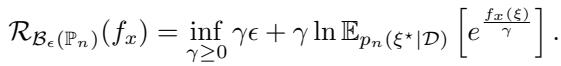
The Bad: The posterior predictive distribution often takes a complex form. For example, if you have a Gaussian likelihood and a Gamma prior, your predictive distribution is a Student-t distribution. Calculating the Moment Generating Function (MGF)—the term \(\mathbb{E}[e^{f_x}]\) seen in the equation above—for a Student-t distribution is often impossible because it doesn’t exist or is infinite. This forces us to approximate the distribution using sampling (Sample Average Approximation), which reintroduces estimation errors.

2. BAS via Posterior Expectation (DRO-BAS\(_{PE}\))

This is the paper’s primary contribution. Instead of centering the ball on the predictive distribution, BAS\(_{PE}\) defines the ambiguity set based on the expected distance to the model family.

Here, the ambiguity set \(\mathcal{A}_\epsilon(\Pi)\) contains all distributions \(\mathbb{Q}\) such that the average KL divergence from \(\mathbb{Q}\) to the parametric models \(\mathbb{P}_\theta\) (weighted by the posterior) is small.

This might sound more abstract, but it has a “magical” property when dealing with the Exponential Family of distributions.

The Exponential Family Advantage

The Exponential Family includes many of the most common distributions in statistics: Normal (Gaussian), Exponential, Gamma, Beta, Bernoulli, and Poisson.

When the likelihood model belongs to the exponential family and we use a conjugate prior, the math simplifies beautifully. The authors prove that for these models, the complex optimization problem collapses into a single-stage stochastic program.

Specifically, if the conditions are met (conjugate priors and exponential likelihoods), the worst-case risk can be calculated exactly without needing nested sampling loops.

The general dual formulation for BAS\(_{PE}\) is:

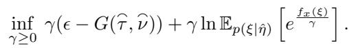
Notice the term \(G(\hat{\tau}, \hat{\nu})\). This is a constant derived from the posterior parameters. Because we can calculate this analytically for exponential families, we don’t need to estimate it.

A Concrete Example: Linear Objective with Gaussian Model

To see the power of BAS\(_{PE}\), consider a scenario where your objective function is linear (like minimizing portfolio cost) and your data is Gaussian.

If you use DRO-BAS\(_{PE}\), the optimization problem becomes a closed-form equation:

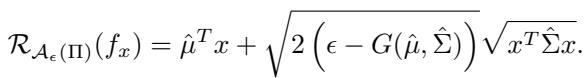
Here:

• \(\hat{\mu}\) and \(\hat{\Sigma}\) are the posterior mean and covariance.
• \(G(\dots)\) is a calculated constant based on your uncertainty.
• \(x\) is your decision variable.

There are no integrals, no Monte Carlo samples, and no loops. You plug this equation into a standard solver, and it gives you the optimal, robust decision instantly. This is a massive computational advantage over BDRO.

Experimental Results

Theory is great, but does it work? The authors tested these methods on two classic problems: the Newsvendor problem (inventory management) and Portfolio Optimization.

1. The Newsvendor Problem

In this problem, a retailer must decide how much inventory (\(x\)) to stock to meet uncertain demand (\(\xi\)). Stock too much, and you lose money on holding costs. Stock too little, and you lose potential sales.

The authors compared the methods on “Out-of-Sample” (OOS) performance. They trained the decisions on small datasets and tested them on unseen data. They plotted the Mean vs. Variance of the costs. Ideally, you want to be in the bottom-left corner (low cost, low variance).

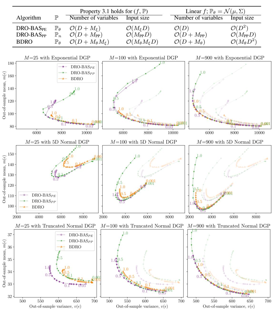
Figure 2 above illustrates the results across different Data Generating Processes (DGPs).

• The Purple Dotted Line (DRO-BAS\(_{PE}\)) consistently forms the “Pareto Frontier” (the optimal boundary). It dominates the other methods, offering lower risk for the same return.
• The Orange Line (BDRO) requires significantly more samples (\(M=900\)) to even approach the performance that DRO-BAS achieves with fewer resources.
• Notice the middle row (Normal DGP): BAS\(_{PE}\) is strictly better (lower and to the left) than BDRO.

2. The Portfolio Problem

Here, the goal is to allocate wealth across assets to maximize return (or minimize negative return) while managing risk. The data is real-world weekly stock returns from the Dow Jones index.

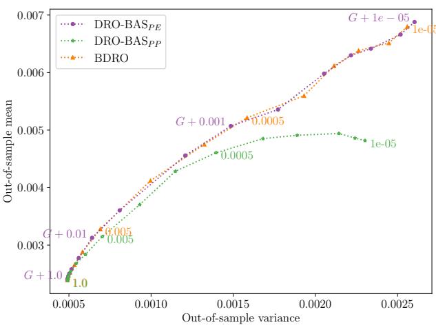
In Figure 3, we see the mean-variance tradeoff.

• DRO-BAS\(_{PE}\) (Purple) and BDRO (Orange) perform similarly in terms of robustness.
• DRO-BAS\(_{PP}\) (Green) struggles here, likely because the Student-t predictive distribution forces the use of sampling approximations that degrade performance.

However, the real differentiator here is speed.

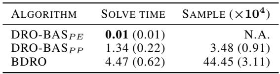
Table 2 reveals the computational gap.

• DRO-BAS\(_{PE}\) solves in 0.01 seconds.
• BDRO takes 4.47 seconds.

That is a 400x speedup. In high-frequency trading or real-time logistics, that difference is critical. BDRO is slow because it has to sample covariance matrices from an Inverse-Wishart distribution and solve a two-stage problem. DRO-BAS\(_{PE}\) just solves a single analytical equation.

Conclusion & Takeaways

The paper “Decision Making under the Exponential Family” provides a compelling argument for rethinking how we handle uncertainty in optimization.

Here are the key takeaways for students and practitioners:

1. Don’t Average the Worst Cases: The existing BDRO method averages the worst-case risks of many models. It’s conceptually messy and computationally slow.
2. Use the Structure of Your Model: By leveraging the mathematical properties of the Exponential Family and Conjugate Priors, DRO-BAS\(_{PE}\) turns a seemingly intractable robust optimization problem into a fast, single-stage convex program.
3. Speed + Robustness: You don’t always have to trade computational speed for better results. DRO-BAS\(_{PE}\) dominates on both fronts for applicable models.
4. The “PE” Formulation is Superior: While the Posterior Predictive (PP) approach makes intuitive sense, the Posterior Expectation (PE) approach yields better mathematical properties (convexity, closed-form duals) and empirical results.

This work bridges the gap between Bayesian Statistics (which quantifies what we know) and Robust Optimization (which protects us from what we don’t). For anyone building decision systems on limited data, “hedging your bets” with Bayesian Ambiguity Sets looks like the winning strategy.

---