](https://deep-paper.org/en/paper/2412.03719/images/cover.png)
If you have ever built an application on top of a Large Language Model (LLM), you have likely encountered behavior that feels inexplicably brittle. You construct a carefully worded prompt, get a great result, and then—perhaps accidentally—you add a single trailing whitespace to the end of your prompt. Suddenly, the model’s output changes completely.
Why does a system capable of passing the bar exam stumble over a space bar?
The answer lies in a fundamental disconnect between how humans read text and how modern LLMs process it. Humans see characters; models see tokens. This disconnect creates what researchers call the Prompt Boundary Problem.
In this post, we will dive deep into a recent paper, “From Language Models over Tokens to Language Models over Characters,” which proposes a mathematically principled solution to bridge this gap. We will explore how to convert token-level probabilities into character-level probabilities, allowing for robust, predictable text generation that isn’t derailed by a stray space.
The Root of the Problem: Tokens vs. Characters
To understand the problem, we first need to look at how an LLM sees the world. An LLM does not define a probability distribution over strings of characters (like “a”, “b”, “c”). Instead, it operates on a vocabulary of tokens (integers), produced by a tokenizer like Byte-Pair Encoding (BPE).
When you feed the string “In the kingdom” into a model, it is first chopped into chunks.
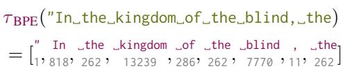
As shown above, the tokenizer converts the character string into a specific sequence of integers. The model then predicts the next integer.
The Prompt Boundary Problem
The tension arises because there are often multiple ways to tokenize a string, but the model is usually trained and queried using a single “canonical” tokenization.
Consider the prompt: "In_the_kingdom_of_the_blind,_the" (where _ represents a space).
If we ask the model to complete this proverb using greedy decoding (taking the most likely next token), it correctly predicts _one (token ID 530), leading to “In the kingdom of the blind, the one-eyed man is king.”
However, if we tweak the prompt ever so slightly by adding a trailing space—"In_the_kingdom_of_the_blind,_the_"—the tokenization changes. The final token is no longer the (token 262); it might become _the combined with the space, or the space might become its own token _ (token 220).
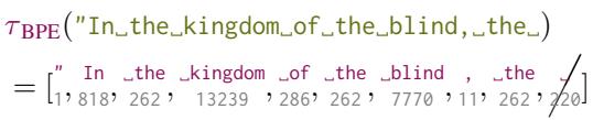
In the paper’s example using GPT-2, adding that whitespace drops the probability of the target word significantly. The model no longer predicts “one”. Instead, it predicts “ills”, resulting in: “…the ills of the world…”
This is the Prompt Boundary Problem. By forcing the model to commit to a specific tokenization of the prompt before it generates the completion, we lock it into a path that might not represent the most probable continuation of the characters.
Why “Token Healing” Isn’t Enough
Engineers have developed heuristics to patch this. The most common is Token Healing. The idea is simple: before generating, you delete the last token of the prompt and let the model re-generate it along with the completion. This allows the model to “heal” the boundary between the prompt and the new text.
While effective for simple cases, token healing fails when a single word is split across multiple tokens in a way that backing up one step cannot fix.
Consider the prompt: "Hello, _worl".
You want the model to complete this to "Hello, _world".
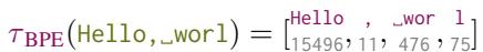
As seen in the figure above, the tokenization for “world” might be split awkwardly. If the prompt ends in worl, the tokenizer might output [Hello, _, wor, l]. Backing up one token (l) isn’t enough to help the model realize it should have output the token world. The model is stuck in a low-probability path in the token space, even though the character sequence is very common.
The Solution: A Covering
The authors propose a rigorous solution: instead of hacking the prompt, we should mathematically translate the model’s token probabilities into character probabilities.
We want to calculate \(p_{\Sigma}(\sigma)\), the probability of a character string \(\sigma\). Since the model gives us \(p_{\Delta}(\delta)\), the probability of a token string \(\delta\), we need a way to map between them.
The challenge is that a single character string can be represented by many different token sequences. For example, the character “a” could be the token a, or part of the token apple, or part of cat.
Defining the Covering
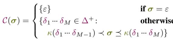
To solve this, the authors introduce the concept of a Covering.
For a target character string \(\sigma\), the covering \(\mathcal{C}(\sigma)\) is the set of all token sequences that:
- Decode to a string that starts with \(\sigma\).
- Are “minimal”—meaning if you remove the last token, they no longer cover \(\sigma\).
Think of the covering as a “frontier” in the token space. It represents every possible valid way the model could have started generating the characters in your prompt.
For the string “Hello, worl”, the covering would include:
[Hello, _, world](Matches “Hello, world”, which starts with “Hello, worl”)[Hello, _, wor, ld][Hell, o, _, world]
Crucially, the covering accounts for the fact that the token generation process might be “mid-token” relative to the character string.
From Token Probabilities to Character Probabilities
Once we have the set \(\mathcal{C}(\sigma)\), we can calculate the prefix probability of the character string. This is the total probability mass of all token sequences in the covering.
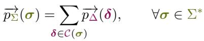
This equation is the bridge. It says: “The probability of the character string \(\sigma\) is the sum of the probabilities of every minimal token sequence that creates \(\sigma\).”
By computing this sum, we marginalize over all possible tokenizations. It doesn’t matter if the model “prefers” one specific tokenization; if the aggregate probability of all valid tokenizations is high, the character string is considered probable.
This effectively solves the prompt boundary problem. Whether you type “the” or “the “, the algorithm looks at all token sequences compatible with those characters, neutralizing the brittleness of the specific tokenizer.
The Algorithms
Calculating this sum exactly is computationally expensive because the number of possible token sequences can grow exponentially with the length of the string. However, the authors present algorithms to approximate this efficiently.
Recursive Enumeration with Pruning
The core algorithm, enum_cover, recursively builds token sequences. It starts with an empty sequence and tries adding every token in the vocabulary.
- Append a token.
- Decode the sequence to characters.
- Check: Does it match the target character string \(\sigma\)?
- If it diverges (e.g., target is “Hel” and we generated “Ha”), discard it.
- If it matches exactly or is a prefix, keep going.
- If it covers the target (is longer than \(\sigma\)), add it to the covering set.
Because the vocabulary is large (often 50k+ tokens), checking every token at every step is too slow. The authors use a Beam Search heuristic to prune the search space.
At each step, they only keep the top-\(K\) most probable token sequences (the “beam”). This assumes that the vast majority of probability mass is concentrated in a few likely tokenizations, which is generally true for natural language.
Bundled Beam Summing
To make this even faster, the researchers implemented a “Bundled” approach. Instead of tracking individual token sequences, they group sequences that are conceptually similar into bundles.
They use a Trie (prefix tree) to efficiently query the language model for valid next tokens. This allows them to filter out thousands of invalid tokens (those that don’t match the next character in the target string) in bulk, rather than iterating one by one.
This optimization allows the algorithm to run in linear time with respect to the length of the character string, making it feasible for real-time applications.
Experimental Results
The authors tested their method on four open-source models (including Llama-3 and Phi-4) using the Wikitext-103 dataset. They aimed to answer two main questions:
- Accuracy: How close is the beam search approximation to the “true” distribution?
- Performance: Is it fast enough?
Accuracy vs. Speed
They measured the Jensen-Shannon Distance (JSD) between their approximation (with small beam sizes) and a high-fidelity reference model (beam size \(K=128\)).
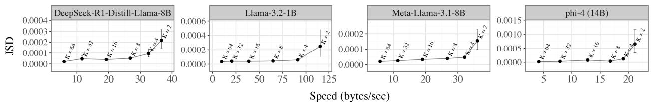
The results in Figure 1(a) show a clear trade-off. As the beam size (\(K\)) increases (moving left on the X-axis), the error drops significantly.
- Speed: Small beam sizes (right side of the curves) are very fast, processing over 100 bytes/sec for smaller models.
- Convergence: The error flattens out quickly. A beam size of \(K=8\) or \(K=16\) provides a very accurate approximation of the true character distribution, with diminishing returns for larger beams.
Improving Compression (Surprisal)
One of the most interesting findings is how this method affects surprisal. Surprisal (measured in bits/byte) essentially measures how well a model predicts text. Lower surprisal means better prediction/compression.
The standard way to evaluate LLMs uses “canonical tokenization”—forcing the model to evaluate the specific token sequence the tokenizer outputs.
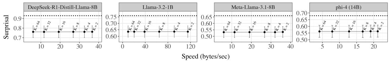
In Figure 1(b), the dotted horizontal line represents the baseline surprisal using canonical tokenization. The data points represent the character-level method.
The character-level method consistently achieves lower surprisal.
Why? Because canonical tokenization is arbitrary. Sometimes a “typo” or a strange word split in token space actually represents the correct character sequence. By summing over all possible tokenizations (via the covering), the model gets “credit” for valid predictions that the canonical tokenizer would have penalized. This suggests that LLMs are actually better models of text than we thought—we were just evaluating them through a restrictive lens.
Conditional Generation
Finally, the paper provides an algorithm for conditional token generation. This replaces the standard generation loop.
\[p_{\Delta|\Sigma}(\delta | \sigma) \stackrel{\text{def}}{=} \mathbb{P}_{Y \sim p_{\Delta}} [ Y = \delta \mid \kappa(Y) \succeq \sigma ]\]Instead of just sampling the next token, the algorithm:
- Enumerates the covering of the prompt \(\sigma\).
- Samples a token sequence \(\delta\) from the covering proportional to its probability.
- Continues generating from there.
This guarantees that the generation is mathematically consistent with the character prompt, effectively solving the prompt boundary problem illustrated at the start of this post.
Conclusion
The shift from “tokens” to “characters” might seem like a semantic detail, but it addresses a major usability flaw in Large Language Models. The Prompt Boundary Problem—where a trailing space changes the output—is a symptom of the mismatch between the model’s internal representation and the user’s input.
By treating the LLM as a distribution over characters (computed by marginalizing over tokens), the authors provide a way to interface with these models that is:
- Robust: No more trailing-space bugs.
- Principled: Based on probability theory, not heuristics like token healing.
- Better: actually results in lower surprisal scores.
For students and researchers, this paper serves as a reminder that the “standard” way of doing things (canonical tokenization) is often just a convenience, not a ground truth. Digging into the mathematical foundations often reveals better, more robust ways to use these powerful tools.