Why Diffusion Models Memorize: A Geometric Perspective and How to Fix It

Generative AI has seen a meteoric rise, with diffusion models like Stable Diffusion and Midjourney creating stunning visuals from simple text prompts. However, beneath the impressive capabilities lies a persistent and potentially dangerous problem: memorization.

Occasionally, these models do not generate new images; instead, they regurgitate exact copies of their training data. This poses significant privacy risks (e.g., leaking medical data or private photos) and copyright challenges. While researchers have proposed various heuristics to detect this, we have lacked a unified framework to explain why it happens mathematically and where it occurs in the model’s learned distribution.

In a recent paper presented at ICML 2025, researchers introduced a geometric framework to analyze memorization through the “sharpness” of the probability landscape. They discovered that memorized samples reside in sharp, narrow peaks of the probability distribution. Leveraging this insight, they developed a method to detect memorization before the image generation process even begins and a strategy to prevent it without retraining the model.

In this post, we will break down the geometry of memorization, explore the mathematics of “sharpness,” and explain how we can steer diffusion models toward safer, more creative outputs.

The Core Intuition: Probability Landscapes

To understand memorization, we must first look at how diffusion models view data. A diffusion model learns a probability distribution \(p(\mathbf{x})\). High-probability regions correspond to realistic images, while low-probability regions correspond to noise or unrealistic data.

You can imagine this learned distribution as a landscape.

• Generalized samples (creative, novel images) reside on broad, smooth hills. There is room for variation; moving slightly in any direction still results in a valid, realistic image.
• Memorized samples (exact training data copies) reside on sharp, narrow peaks. The model has “overfit” to these specific points, creating a steep spike in the probability density.

The researchers propose that by measuring the curvature (sharpness) of this landscape, we can distinguish between creativity and regurgitation.

Background: The Score and The Hessian

Diffusion models generate data by following the “score function,” which points toward higher data density. The reverse diffusion process is governed by stochastic differential equations (SDEs), as shown below:

Here, \(\nabla_{\mathbf{x}_t} \log p_t(\mathbf{x}_t)\) is the score function. It tells the model which direction to move to denoise the image.

To measure sharpness, we look at the derivative of the score function, known as the Hessian Matrix (\(H\)).

• The Score is the slope of the landscape.
• The Hessian describes the curvature of the landscape.

Mathematically, the eigenvalues of the Hessian tell us about the local geometry. Large negative eigenvalues indicate a sharp peak (concavity), meaning the data point is isolated and likely memorized. Small or positive eigenvalues indicate a flatter, smoother region, suggesting generalization.

Visualizing Memorization

The authors validated this geometric hypothesis using a simple 2D toy experiment and MNIST digits.

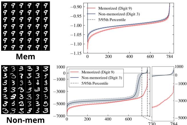
In the figure above, the model was trained to memorize the digit “9” (by repeating it in the dataset) while generalizing the digit “3”.

• Top Right (Initial Step): Even at the very beginning of the generation process (pure noise), the “memorized” trajectory (Red) shows different eigenvalue characteristics than the “generalized” one (Blue).
• Bottom Right (Final Step): The difference becomes stark. The memorized sample has a distribution of eigenvalues with a long tail of large negative values. This confirms that memorized samples sit atop sharp geometric peaks.

This behavior isn’t just limited to simple datasets. We see the exact same evolution in complex models.

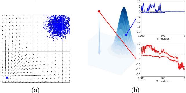
As shown in Figure 1(b) above, the memorized sample (red line) dives deep into negative eigenvalue territory as the generation progresses (\(t \to 0\)), whereas the non-memorized sample (blue line) stays relatively flat.

Measuring Sharpness Efficiently

Calculating the full Hessian matrix for a high-dimensional image (like a 512x512 pixel output from Stable Diffusion) is computationally intractable. It requires calculating second-order derivatives for millions of parameters. We need a shortcut.

The Score Norm Proxy

The researchers utilize a clever mathematical identity connecting the norm of the score (the magnitude of the gradient) to the trace of the Hessian (the sum of eigenvalues).

In simple terms, regions with steep slopes (high score norm) usually correspond to regions with sharp curvature (high negative Hessian trace). This allows us to use the score norm—which is easy to compute—as a proxy for sharpness.

Reinterpreting Existing Metrics

This geometric framework provides a theoretical backbone for previous heuristic methods. For example, a popular detection metric by Wen et al. (2024) measures the difference between the conditional score (with text prompt) and the unconditional score (no prompt):

Why does this work? The researchers prove that this metric effectively measures the difference in sharpness introduced by the text prompt.

As the equation above shows, Wen’s metric is mathematically equivalent to summing the squared differences of the eigenvalues (\(\lambda\)) of the conditional and unconditional Hessians.

We can visualize this gap in Figure 5:

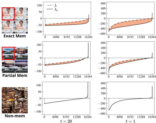
For memorized samples (Exact Mem), the conditional Hessian (\(\lambda_c\)) diverges significantly from the unconditional one (\(\lambda\)). The text prompt effectively forces the model into a sharp, narrow valley corresponding to the training data. For non-memorized samples, the conditioning doesn’t drastically alter the landscape’s curvature.

Early Detection via Hessian Upscaling

While Wen’s metric works well at intermediate steps, detection is difficult at the very start of the diffusion process (\(t=T\)). At this stage, the image is almost pure noise, and the probability landscape is nearly isotropic (uniform in all directions). The “sharpness” signal is weak.

To solve this, the authors propose a new metric that “upscales” the curvature signal. Instead of just looking at the score, they look at the score multiplied by the Hessian.

By projecting the score onto the Hessian, they amplify the components corresponding to large eigenvalues (the sharpest directions). The resulting detection metric is:

This metric acts like a magnifying glass for curvature. It makes the distinction between memorized and non-memorized samples obvious even at the very first timestep.

Detection Results

The results of this new metric are impressive. Table 1 compares detection performance (AUC) on Stable Diffusion.

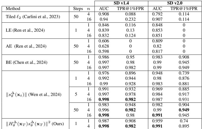
The proposed metric (bottom row) achieves an AUC of 0.998 using only the information available at step 1 (\(t=T-1\)). This means we can flag a potential copyright violation before the model generates a single pixel of the image.

Mitigation: Sharpness-Aware Initialization (SAIL)

If we can detect that a specific starting noise vector \(\mathbf{x}_T\) will lead to a memorized image, can we simply change the starting point?

This is the premise of SAIL (Sharpness-Aware Initialization for Latent Diffusion).

The Logic of SAIL

Since diffusion ODE solvers are deterministic, the initial noise \(\mathbf{x}_T\) completely determines the final image. Memorized images come from initialization noise that sits in “sharp” regions of the latent space.

SAIL solves an optimization problem at inference time. It searches for a new starting noise vector \(\mathbf{x}_T\) that:

1. Minimizes the sharpness (using the Hessian-based metric).
2. Stays close to the standard Gaussian distribution (to ensure the image remains realistic).

The objective function is:

Because calculating the exact Hessian is slow, they use a finite difference approximation, making the process efficient enough for real-time use:

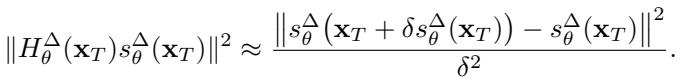
Results: Quality vs. Safety

Most existing mitigation methods try to fix memorization by altering the text prompt (e.g., adding random tokens) or suppressing the attention mechanism. This often breaks the image, changing the subject or style significantly.

SAIL, however, only changes the noise. It keeps the prompt and the model weights exactly the same.

Quantitative Results:

In Figure 6 (Left), we see that SAIL (Red/Pink lines) achieves the best balance: low memorization scores (SSCD) and high image-text alignment (CLIP).

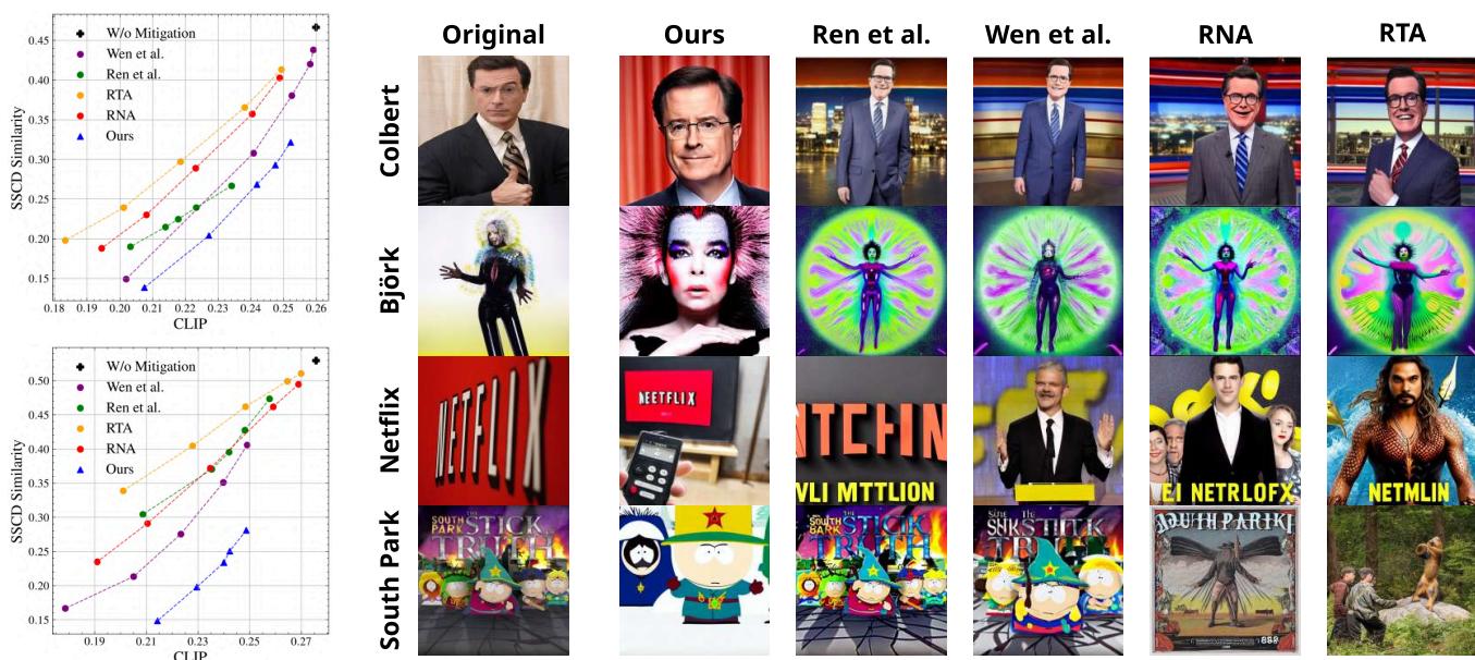
Qualitative Results:

The visual difference is striking. In the example below, the goal is to generate an image based on a prompt that originally triggered a memorized output (like a specific celebrity photo or movie scene).

• Original: Shows the memorized training image.
• Ours (SAIL): Generates a high-quality image of the correct subject (e.g., Anne Hathaway, Ricky Gervais) that respects the prompt but is not a copy of the training data.
• Baselines (Ren et al., Wen et al., etc.): Often distort the face, change the background to something unrelated, or ruin the composition in an attempt to hide the memorization.

Conclusion

This research offers a compelling new way to think about generative AI. Memorization isn’t just a “bug” of the dataset; it’s a geometric feature of the probability landscape that the model learns.

By mathematically characterizing this geometry via the Hessian and its eigenvalues, the authors provided:

1. A theoretical explanation for why existing metrics work.
2. A superior detection metric that identifies privacy risks at the very first step of generation.
3. SAIL, a mitigation strategy that fixes the problem at the source (the initialization noise) rather than applying band-aids to the prompt.

As we move toward deploying generative models in sensitive fields like healthcare and creative industries, tools like SAIL will be essential for ensuring these systems are safe, private, and truly creative.