The Return of the Flow: How TARFLOW Makes Normalizing Flows Competitive with Diffusion

If you have been following the generative AI landscape over the last few years, the narrative seems clear: Diffusion Models (like Stable Diffusion or DALL-E) and Autoregressive Models (like GPT-4) have won. They generate the highest quality images and text, dominating the leaderboards.

Meanwhile, Normalizing Flows (NFs)—a family of models known for their elegant mathematical properties—have largely been left behind. While they were once a popular choice for density estimation, they gained a reputation for being computationally expensive and unable to produce the high-fidelity samples we see from diffusion models.

But what if Normalizing Flows aren’t inherently limited? What if we just haven’t been training them correctly?

In a new paper titled “Normalizing Flows are Capable Generative Models,” researchers from Apple demonstrate that NFs are significantly more powerful than previously believed. They introduce TARFLOW, a Transformer-based architecture that achieves state-of-the-art results in image likelihood estimation and generates samples that rival diffusion models.

In this post, we will break down how TARFLOW works, the specific architectural changes that make it scalable, and the clever training techniques—like “denoising” and “guidance”—that unlock its full potential.

The Problem with Normalizing Flows

To understand why TARFLOW is significant, we first need to understand the premise of Normalizing Flows.

A Normalizing Flow is a generative model that learns an invertible mapping \(f\) between a complex data distribution \(x\) (like images) and a simple prior distribution \(z\) (usually a standard Gaussian, or “noise”).

The training objective is Maximum Likelihood Estimation (MLE). Because the mapping is invertible, we can compute the exact likelihood of the data using the Change of Variable formula:

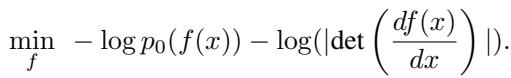
If we assume the prior \(p_0\) is a standard Gaussian, the objective simplifies to minimizing two terms:

1. The Norm Term (\(0.5 \|f(x)\|^2_2\)): Encourages the model to map data samples to latent vectors with small norms (keeping them close to the center of the Gaussian).
2. The Jacobian Term (\(-\log |\det|\)): Prevents the model from “collapsing” (mapping different inputs to the same output) and encourages it to spread out over the latent space.

Why have they struggled?

Despite these nice mathematical properties, NFs have struggled with scalability. Previous architectures (like RealNVP or Glow) relied on specific “coupling layers” designed to make the Jacobian determinant easy to compute. However, these designs often restricted the model’s expressiveness. Conversely, methods that were more expressive (like Neural ODEs) were often numerically unstable or slow to train.

TARFLOW challenges this status quo by combining the flow framework with the most successful architecture in modern deep learning: the Transformer.

The TARFLOW Architecture

The core of TARFLOW is the Block Autoregressive Flow.

Autoregressive flows (like the older MAF models) typically work pixel-by-pixel. To predict the transformation for pixel \(i\), they look at pixels \(0\) to \(i-1\). TARFLOW generalizes this by working on patches of images, similar to a Vision Transformer (ViT).

From Pixels to Patches

The model treats an image not as a grid of pixels, but as a sequence of patches. If you have an image, it is chopped up into a sequence \(x\). The flow transforms this sequence step-by-step.

The architecture stacks multiple “Flow Blocks.” As shown in the figure below, the process is deep and iterative:

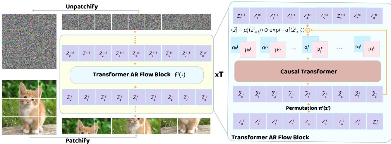
Each Transformer AR Flow Block consists of three main steps:

1. Permutation (\(\pi^t\)): The sequence of patches is reordered. For example, if layer 1 processes the image from top-left to bottom-right, layer 2 might process it in reverse. This allows information to propagate globally across the image.
2. Causal Transformer: A standard causal Transformer (with masked attention) processes the sequence. Because it is causal, the transformation for patch \(i\) depends only on patches preceding it in the current order.
3. Affine Transformation: The output of the Transformer predicts the parameters (\(\mu\) and \(\alpha\)) used to transform the input latent \(z^t\).

The Forward Pass

In the forward pass (going from data to noise), the transformation for the \(t\)-th block looks like this:

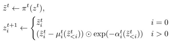
Here, the model predicts a shift (\(\mu\)) and a log-scale (\(\alpha\)) based on previous patches. These are used to normalize the current patch.

The Inverse Pass (Generation)

Generating an image involves reversing this process. We sample noise \(z\) and pass it backward through the layers. The inverse equation is:

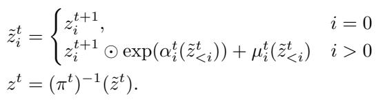
Because the Transformer is causal, we can generate the image patch-by-patch (or block-by-block). We compute the parameters for the first patch, sample it, feed it back into the Transformer to get parameters for the second patch, and so on.

This architecture allows TARFLOW to scale up easily. You can simply add more layers or make the Transformer wider, just like a Large Language Model (LLM).

Three Critical Techniques for Quality

Architecture alone isn’t enough. The authors introduce three specific techniques that take TARFLOW from “mathematically correct” to “visually stunning.”

1. Gaussian Noise Augmentation

In standard flow training, it’s common to add “uniform dequantization noise” (noise roughly the size of a pixel bin) to continuous inputs. This prevents the model from collapsing onto the discrete values of digital images (0, 1, … 255).

However, the researchers found that for perceptual quality, uniform noise isn’t good enough. Instead, they add Gaussian noise with a magnitude (\(\sigma\)) slightly larger than the pixel bin size.

Why? If you don’t add enough noise, the inverse model (generator) is trained on a very sparse set of points (the training images). When you try to generate new images from the continuous Gaussian prior, the model hits “dead zones” where it hasn’t learned meaningful representations. Adding Gaussian noise effectively “smears” the training data, creating a smoother manifold for the model to learn.

2. Score-Based Denoising

There is a catch to adding noise: if you train on noisy images, your model will generate noisy images. The samples will look grainy.

To fix this, the authors borrow a trick from diffusion models and score-based modeling: Tweedie’s Formula.

Tweedie’s formula allows you to estimate the “clean” data point \(x\) given a noisy observation \(y\), provided you know the score (the gradient of the log-likelihood). The formula is:

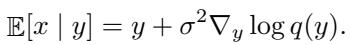
The beautiful part is that a Normalizing Flow calculates the likelihood explicitly. We already have \(\log p_{\text{model}}(y)\). Therefore, we can denoise the generated sample using the model’s own gradients, without training a separate denoiser!

The complete sampling procedure becomes:

1. Sample noise \(z\) from the prior.
2. Pass it through the flow inverse \(f^{-1}\) to get a noisy image \(y\).
3. Apply the denoising step to get clean image \(x\).

The visual impact of this technique is massive. In the figure below, look at the difference between the “raw samples” (top) and “denoised” (bottom).

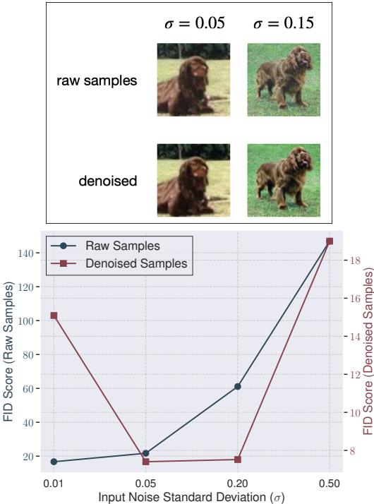
As shown in the graph (bottom of Figure 4), before denoising (blue line), adding more noise hurts quality. After denoising (red line), adding noise actually improves quality, provided you clean it up at the end.

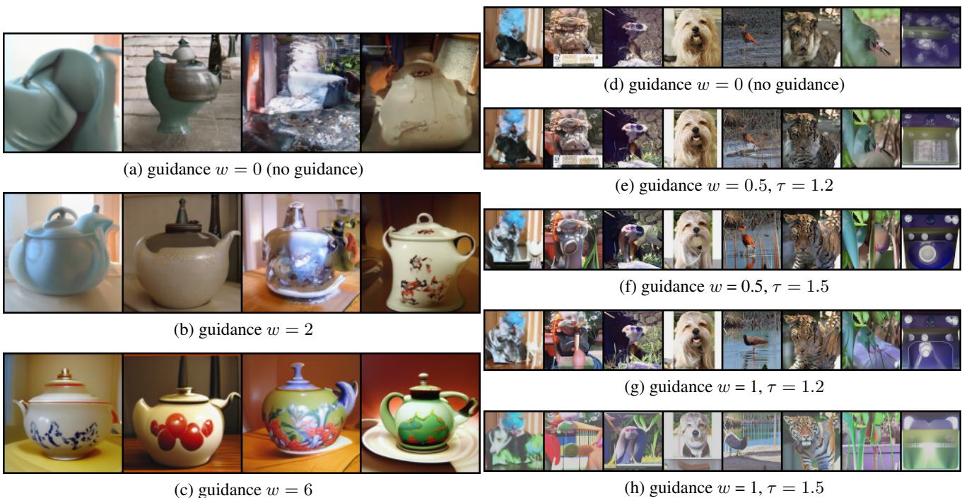
3. Guidance (CFG for Flows)

One of the key features that made text-to-image models popular is Classifier-Free Guidance (CFG). This technique pushes the generation toward a specific class condition (or prompt) and away from a generic, unconditional prediction. It trades diversity for fidelity.

The authors show that Guidance works for Normalizing Flows too.

They modify the inverse flow step. Instead of using the predicted \(\mu\) and \(\alpha\) directly, they compute a “guided” version. This is done by taking the difference between a conditional prediction (e.g., “dog”) and an unconditional prediction (empty context), and amplifying it by a weight \(w\).

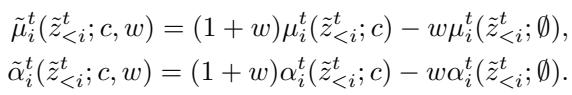
Visually, increasing the guidance weight \(w\) transforms vague, noisy blobs into sharp, recognizable objects.

Experimental Results

So, how does TARFLOW stack up against the competition?

Likelihood Estimation

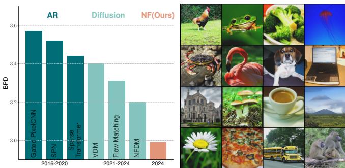
Likelihood (measured in Bits Per Dimension, or BPD) is the “purest” measure of how well a probabilistic model fits the data. Lower is better.

TARFLOW achieves state-of-the-art results on ImageNet 64x64, breaking the 3.0 BPD barrier for the first time. It significantly outperforms previous flows (like Glow and Flow++) and even beats modern Diffusion/Flow Matching models in terms of raw density estimation.

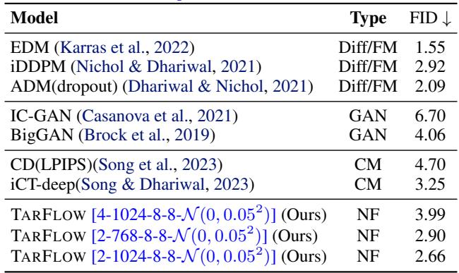
Image Generation

While likelihood is great for science, we care about pretty pictures. The standard metric for image realism is the Fréchet Inception Distance (FID) (lower is better).

Using the techniques described above (Gaussian noise + Denoising + Guidance), TARFLOW produces samples that are competitive with diffusion models.

Interestingly, the sampling process of TARFLOW visually resembles that of a diffusion model. Because it builds the image patch-by-patch (or via iterative refinement in the latent space), you can watch the image emerge from the noise.

Why This Matters

For years, the research community assumed that Normalizing Flows were inherently limited in their generative capabilities compared to Diffusion models. This paper suggests that the gap wasn’t fundamental—it was architectural and methodological.

By adopting the Transformer backbone (scalability), identifying the importance of Gaussian noise (smoothing the manifold), and implementing Score-Based Denoising (cleaning the output), TARFLOW brings NFs back into the conversation.

This is exciting because NFs offer properties that diffusion models don’t, such as exact likelihood computation and a deterministic mapping between data and latents. With TARFLOW, we might see a resurgence of flow-based models in high-fidelity generation tasks.

Key Takeaways:

• Architecture: Transformers work everywhere, including Normalizing Flows.
• Noise Strategy: Gaussian noise during training is better than uniform noise for perception, but requires a denoising step.
• Denoising: You can “self-correct” a flow model’s output using its own likelihood gradients.
• Guidance: Classifier-Free Guidance isn’t just for diffusion; it boosts flow fidelity significantly.

TARFLOW proves that with the right design choices, the “forgotten” family of generative models is capable of state-of-the-art performance.