](https://deep-paper.org/en/paper/2412.12276/images/cover.png)
Introduction
One of the most fascinating capabilities of Large Language Models (LLMs) is In-Context Learning (ICL). You give a model a few examples—like “Apple -> Red, Banana -> Yellow”—and suddenly, without any weight updates or retraining, it understands the pattern and predicts “Lime -> Green.” To us, this feels intuitive. To a machine learning researcher, it is mathematically perplexing. How does a static set of weights adapt to a new task on the fly?
Recent research has suggested that Transformers represent these tasks as “vectors” inside their hidden states. Think of it as a coordinate in the model’s brain that represents “Translation” or “Sentiment Analysis.” But knowing that these vectors exist doesn’t explain how they get there or why they work better for some tasks than others.
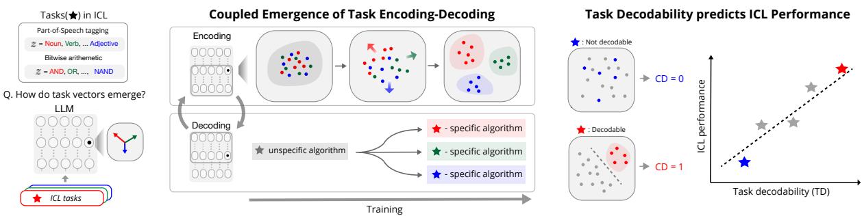
In this post, we are doing a deep dive into the paper “Emergence and Effectiveness of Task Vectors in In-Context Learning: An Encoder Decoder Perspective.” This research peels back the layers of the Transformer to reveal a two-step mechanism: Task Encoding (identifying the task) and Task Decoding (executing the algorithm).
We will explore how models separate distinct concepts in their “mind” during training, why finetuning the first few layers is actually more effective than the last, and how we can mathematically predict a model’s performance just by looking at the geometry of its internal representations.
The Background: ICL as Bayesian Inference
To understand the mechanics, we first need to look at the theoretical framework. The researchers adopt a Bayesian view of In-Context Learning.
Imagine you are looking at a sequence of numbers: 2, 4, 6… and you need to guess the next one.
- First, you unconsciously infer the latent concept (\(z\)): “The rule is even numbers.”
- Second, you apply that rule to generate the prediction (\(y\)): “The next number is 8.”
The paper argues that Transformers implement this exact two-stage process. Mathematically, it looks like this:
Here, \(P_\theta(z | \mathcal{D})\) represents the Task Encoding phase: the model looks at the context examples (\(\mathcal{D}\)) and figures out the latent task \(z\). Then, \(P_\theta(y_* | x_*, z)\) represents the Task Decoding phase: the model uses that task information (\(z\)) to generate the correct output \(y_*\).
The researchers hypothesize that this isn’t just a mathematical abstraction—it is physically happening inside the neural network’s layers. The model encodes the task into a specific vector (representation) and then “decodes” that vector to trigger a specific algorithm.
The Core Method: Investigating Synthetic Tasks
To prove this theory, the authors started with a controlled environment. They trained a small Transformer (GPT-2 architecture) on a Mixture of Sparse Linear Regression tasks.
In plain English: The model was shown sequences of numbers generated by different hidden mathematical rules (bases). Its job was to figure out which rule was being used and predict the next number. Because the researchers created the data, they knew exactly which “latent task” was active at any time.
The Coupled Emergence of Encoding and Decoding
What happens inside the model as it learns? The results were striking. The model didn’t learn everything gradually and evenly. Instead, it showed sudden “phase transitions.”

Let’s break down Figure 2 above, which is central to understanding this phenomenon:
- The Loss Curve (Left): Look at the red line (\(B_1\)). The error drops drastically at specific points (marked a, b, c). This indicates the model suddenly “got it.”
- The Geometry (Right): These UMAP plots show the model’s internal representations of the data.
- At point (a): The dots are a mess. The model cannot distinguish between the different mathematical rules.
- At point (b): The orange cluster separates. This coincides with the first drop in loss. The model has learned to distinguish “Task 1” from the others.
- At point (c): All clusters are distinct. The model has fully separated the tasks in its latent space.
This confirms the Task Encoding-Decoding hypothesis. The model can only solve the task (reduce loss) once it has successfully separated the task’s representation from the others. As the encoding becomes clearer (clusters separate), the decoding (performance) improves.
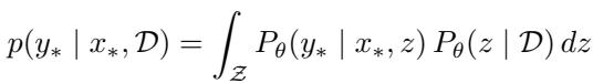
We can see this evolution even more clearly if we look at the representations across layers over time:
In Figure 11, notice Epoch 20. In the early layers (0-3), the representations are mixed. But around Layer 4-5, they start to separate. This suggests the early layers act as the “Encoder,” identifying the task, while the later layers execute the solution.
Moving to Real LLMs: Llama, Gemma, and More
Synthetic data is great for theory, but does this hold up in real Large Language Models? The authors tested this on models ranging from Llama-3.1-8B to Gemma-2-27B, using natural tasks:
- Part-of-Speech (POS) Tagging: (e.g., “Find the noun”).
- Bitwise Arithmetic: (e.g., logical AND, OR, XOR operations).
Measuring “Task Decodability”
To quantify how well a model understands a task, the authors introduced a metric called Task Decodability (TD).
TD is simple: Can a simple classifier (like a k-Nearest Neighbor) look at the model’s hidden state and correctly guess which task (e.g., “Noun” vs. “Verb”) the model is performing?
- High TD: The tasks are well-separated clusters in the model’s brain.
- Low TD: The model is confused; the representations are overlapping.

In Figure 3, look at the difference between Noun (Red) and Preposition (Purple).
- Noun: Forms a tight, distinct cluster. The TD score is high.
- Preposition: Is scattered and overlaps with the “Null” class. The TD score is low.
Crucially, as we provide more “shots” (examples in the prompt), the TD score goes up. The context examples act as a signal that helps the model sharpen its focus and separate the task clusters.
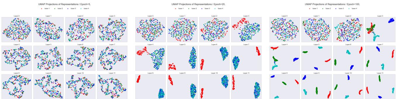
Does High TD Mean Better Performance?
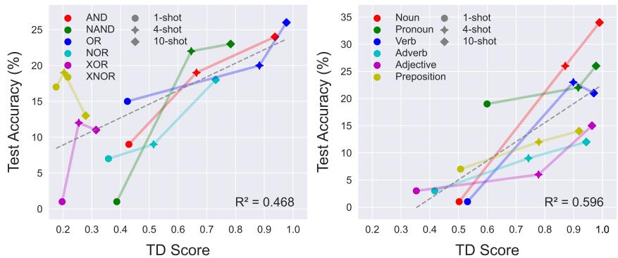
This is the most critical finding for practitioners. There is a near-linear relationship between how well a task is encoded (TD Score) and how well the model performs (Accuracy).
As shown in Figure 4, if the TD score is high, the model is almost guaranteed to have high accuracy. If the TD score is low, the model fails. This suggests that the bottleneck for ICL often isn’t the model’s ability to do the task, but its ability to identify exactly which task you want it to do.
This relationship isn’t unique to Llama. It holds across different model families and sizes, as seen here with Gemma and Llama-70B:

And surprisingly, it even holds for non-Transformer architectures like Mamba (RNNs), suggesting this is a fundamental property of how neural networks learn from context:
Proving Causality: Can We Hack the Task Vector?
Correlation isn’t causation. To prove that these vectors actually cause the model to solve the task, the researchers performed Activation Patching.
They essentially “injected” the task vector for one task (e.g., “AND”) while the model was trying to solve another (or a null task).
- Positive Intervention: Injecting the correct task vector should boost performance.
- Negative Intervention: Injecting the wrong task vector should destroy performance.
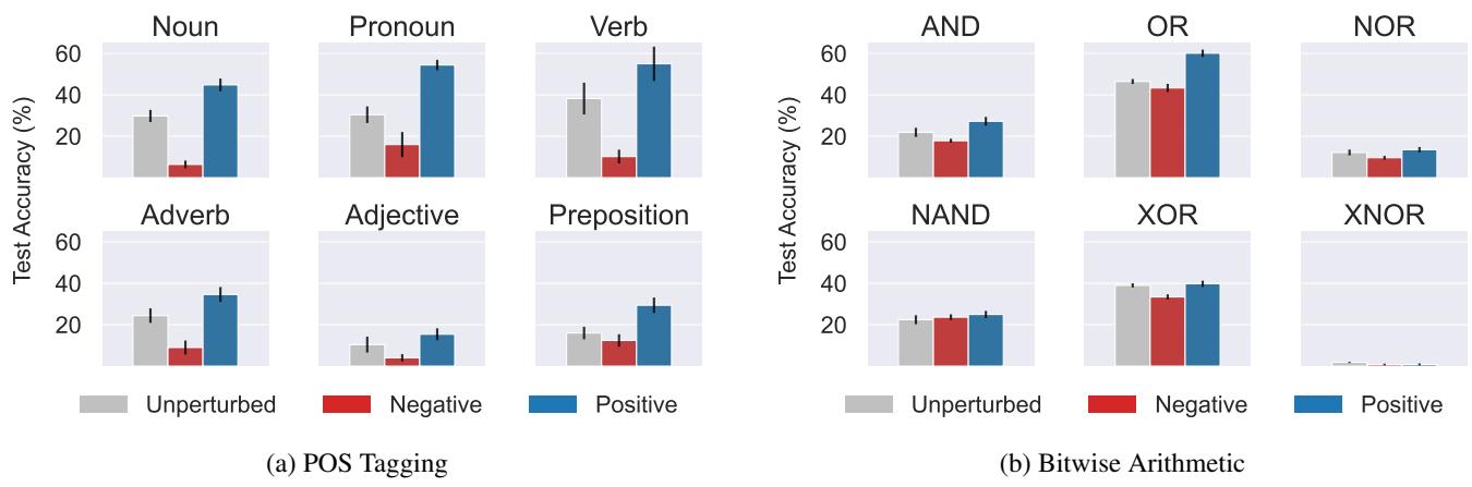
Figure 20 confirms this. Look at the Bitwise Arithmetic chart on the right.
- Grey Bar: Baseline performance.
- Blue Bar (Positive): Performance jumps up (significantly for tasks like AND/OR).
- Red Bar (Negative): Performance crashes.
This confirms that the ICL process is indeed mediated by these geometric task vectors.
The Layer Anatomy: Where Does the Magic Happen?
If the model is an “Encoder-Decoder,” where is the boundary?
The researchers plotted TD scores across the layers of Llama-3.1.
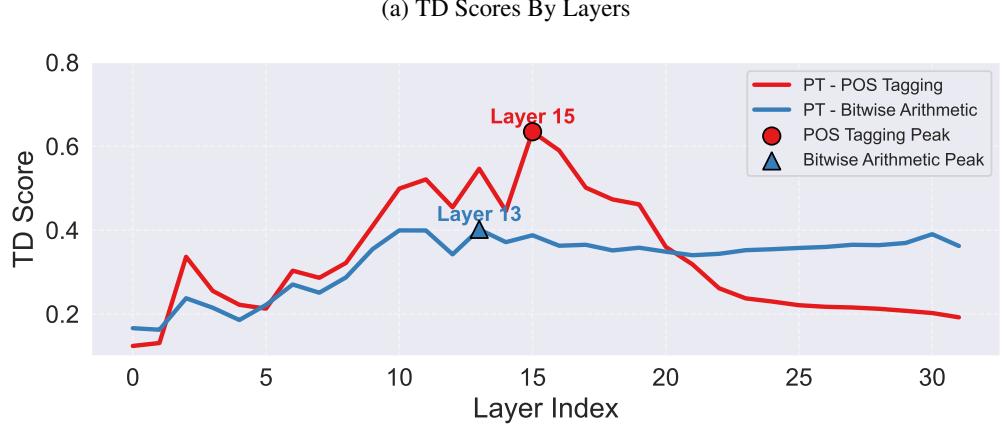
In Figure 19 (a), notice the peak. The ability to identify the task (TD) rises sharply and peaks around Layer 13-15, then drops off.
This implies:
- Early Layers (0-15): The Encoder. These layers are responsible for digesting the prompt and figuring out “What task is this?”
- Late Layers (16+): The Decoder. Once the task is identified, these layers execute the specific algorithm to generate the answer. The task information is “consumed” or transformed into the answer, which is why TD drops.
The Implication: Finetune the Early Layers!
This insight challenges a common convention in Machine Learning. Usually, when we finetune a model (like using LoRA), we focus on the later layers or the prediction head, assuming that’s where the specific knowledge lives.
But if the bottleneck is task identification, we should fix the Encoder.
The researchers tested this by finetuning just the First 10 Layers vs. the Last 10 Layers.
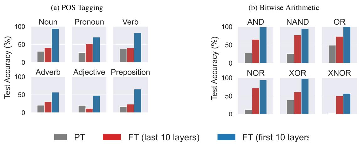
The results in Figure 24 are staggering.
- Blue Bars (First 10 Layers): Massive performance gains.
- Red Bars (Last 10 Layers): Moderate or negligible gains.
For “Bitwise Arithmetic,” finetuning the first 10 layers brought accuracy from near-zero to nearly 100%. By helping the model “see” the task clearly in the early layers, the downstream execution layers could finally do their job.
Evolution During Pretraining
Finally, the paper asks: How does this ability emerge during the massive pretraining run of an LLM? Using checkpoints from the OLMo-7B model, they tracked TD and Accuracy over thousands of training steps.
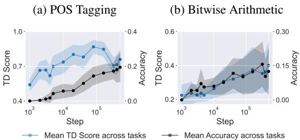
As shown in Figure 5, the two lines track almost perfectly. As the model learns to structure its internal geometry to separate tasks (TD Score rises), its ability to perform In-Context Learning emerges simultaneously.
Conclusion
This research provides a compelling “mechanistic” explanation for the magic of In-Context Learning. It moves us away from viewing LLMs as “black boxes” and towards understanding them as structured engines that perform two distinct operations:
- Task Encoding: Separating latent concepts into distinct geometric clusters in the early layers.
- Task Decoding: Using those specific clusters to trigger algorithmic circuits in the later layers.
Key Takeaways for Students and Practitioners:
- Geometry is predictive: You can predict how well a model will perform on a task just by looking at how well-separated that task’s vector is in the hidden states.
- The “Encoder” is distinct: The early layers of a Transformer are doing the heavy lifting of figuring out what the task is.
- Finetuning Strategy: If your model is struggling to follow instructions or grasp a task, try finetuning the early layers. You might be fixing the “Task Encoder” rather than the execution engine.
As we continue to scale models, understanding why they work is just as important as making them work better. This “Encoder-Decoder” perspective brings us one step closer to fully deciphering the internal language of Large Language Models.