](https://deep-paper.org/en/paper/2412.14363/images/cover.png)
Introduction
The capabilities of Large Language Models (LLMs) like Llama 3 and Qwen2.5 are growing at a staggering pace. However, as these models scale to hundreds of billions of parameters, the computational cost to run them—specifically during inference—is becoming prohibitive. Inference has two main bottlenecks: the compute-bound prefilling stage (processing your prompt) and the memory-bound generation stage (spitting out tokens one by one).
To make these models run on standard hardware (or just run faster on data center GPUs), we rely on quantization—reducing the precision of the model’s numbers from 16-bit floating-point (FP16) to integers like 8-bit or 4-bit. While quantizing weights is relatively solved, quantizing activations (the temporary data flowing through the network) and the KV cache (the model’s memory of the conversation) to 4-bit without turning the model into gibberish remains a massive challenge.
Why? Because of outliers. In LLM activations, a tiny fraction of values are magnitudes larger than the rest. If you try to squeeze these outliers into a tiny 4-bit grid, you either clip them (losing critical info) or stretch the grid so wide that the small, nuanced values get lost in quantization noise.
In this post, we will deep dive into ResQ (Residual Quantization), a new method presented at standard ML conferences that proposes a mathematically optimal way to handle these outliers. By combining mixed-precision quantization with principal component analysis (PCA), ResQ achieves state-of-the-art performance, effectively unlocking accurate 4-bit inference.
The Background: The War on Outliers
Before understanding ResQ, we need to understand the current landscape of quantization.
The Problem
When we quantize a matrix \(X\), we map its continuous values to a discrete set of integers. The standard equation looks like this:
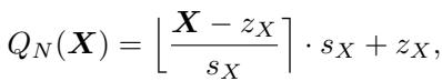
Here, \(s_X\) is the scale factor. If matrix \(X\) has one massive outlier (e.g., 100) while most values are between -1 and 1, \(s_X\) must be large to accommodate the 100. Consequently, the values between -1 and 1 might all get rounded to 0, destroying the signal.
Existing Solutions
Researchers have developed two primary strategies to fight this:
- Mixed-Precision (Outlier Channel Detection): Identify the specific channels (columns/rows) where outliers live and keep them in high precision (e.g., 8-bit or 16-bit), while crunching the rest to 4-bit. The challenge here is: How do you decide which channels are “important”? Most methods just look for the largest values (\(\ell_{\infty}\)-norm).
- Rotation (Uniform Precision): Multiply the activation matrix by a random rotation matrix. This “smears” the outliers across all channels, making the distribution smoother (more Gaussian) and easier to quantize uniformly.
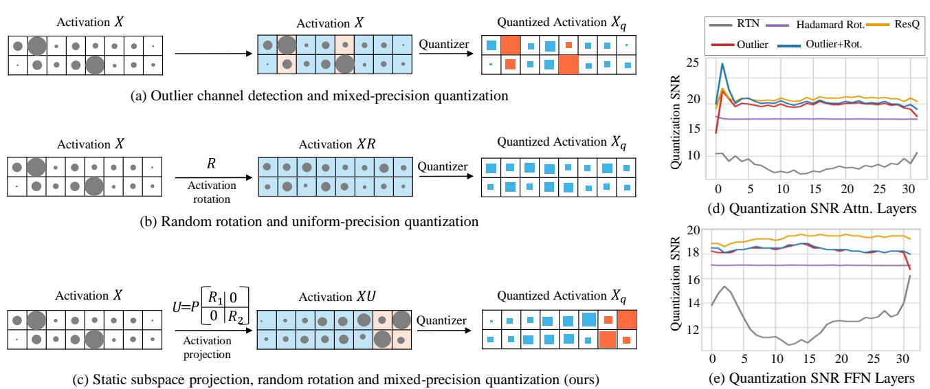
As shown in Figure 1 above, existing methods usually pick one lane. (a) shows outlier detection, where specific high-magnitude channels are kept in orange (high precision). (b) shows rotation, where the data is scrambled to be uniform.
ResQ (c) asks: Why not do both? But specifically, why not use a better metric than just “magnitude” to decide what to keep in high precision?
The Core Method: ResQ
ResQ stands for Residual Quantization. The core philosophy is to identify a “low-rank subspace” that contains the most information (variance), keep that in high precision, and relegate the “residual” (the rest) to low precision. Crucially, it uses invariant random rotations within those subspaces to smooth out the data even further.
The Decomposition
The researchers propose splitting the input activations \(X\) and weights \(W\) using an orthogonal basis \(U\). They split this basis into two parts:
- \(U_h\): The high-precision subspace (rank \(r\)).
- \(U_l\): The low-precision subspace (rank \(d-r\)).
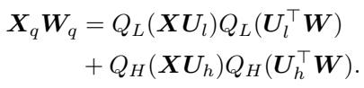
The quantized activation \(X_q\) is calculated as:

This equation says: Project \(X\) into the low-precision space (\(X U_l\)) and quantize it aggressively (\(Q_L\)), then project \(X\) into the high-precision space (\(X U_h\)) and quantize it gently (\(Q_H\)). Sum them up, and you have your result.
Why Orthogonality Matters
You might be wondering, “Doesn’t splitting matrices and multiplying them add massive computational overhead?”
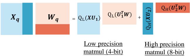
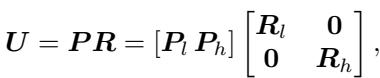
This is where the math gets elegant. Because the basis \(U\) is orthogonal, the cross-terms in the matrix multiplication vanish. When you multiply the quantized activation \(X_q\) by the quantized weight \(W_q\), the operation decomposes cleanly:
This means the hardware only needs to perform a 4-bit GEMM (General Matrix Multiply) for the bulk of the data and an 8-bit GEMM for the small high-precision part. There is no messy interaction between the two precisions.
Figure 2 below illustrates this hardware-friendly flow. Notice how the large blue block (4-bit) and the thin teal block (8-bit) are processed separately and then simply added together.
The Secret Sauce: PCA and Optimality
The most significant contribution of this paper is how they choose the high-precision subspace \(U_h\). Previous methods like QUIK selected channels based on maximum absolute value (magnitude). ResQ uses Principal Component Analysis (PCA).
The authors prove a theorem (Theorem 4.2) demonstrating that to minimize quantization error, you shouldn’t look for the largest values; you should look for the largest variance.
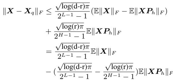
The equation above provides the upper bound of the error. To make the error (LHS) as small as possible, you need to subtract as much as possible on the RHS. This implies maximizing \(\|XP_h\|_F\). In linear algebra, the projection \(P_h\) that maximizes the Frobenius norm of the projected data is exactly the top eigenvectors of the covariance matrix \(XX^T\).
In simple terms: ResQ runs a quick calibration step (using PCA) to find the “directions” in the data that fluctuate the most. It assigns those directions to 8-bit precision. It assigns the boring, static directions to 4-bit.
Adding Rotation
Once the subspaces are identified via PCA, ResQ applies random rotations (\(R_l\) and \(R_h\)) inside those subspaces.
This rotation ensures that within the 4-bit group, no single channel is an outlier, and within the 8-bit group, the data is also well-distributed.
The Effect on Distributions
Does this complex math actually change the data? Yes, dramatically.
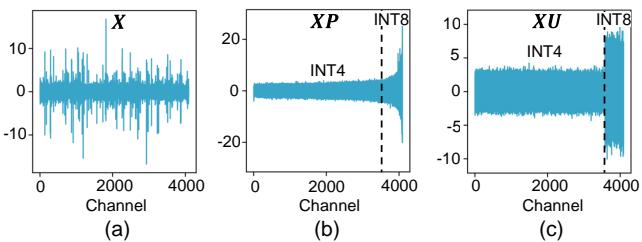
Figure 3 below shows the activation distribution.
- (a) The baseline is jagged and noisy.
- (b) Applying PCA (\(XP\)) sorts the channels by variance. You can see the right side (high variance) spikes up.
- (c) Applying ResQ (\(XU\), which includes rotation) smooths everything out. The “INT4” section is flat and easy to quantize; the “INT8” section captures the heavy lifting.
Implementation in LLM Blocks
Implementing this in a Transformer isn’t as simple as just one matrix multiplication. The projections need to be fused into the weights where possible to avoid slowdowns.
The authors define specific projection matrices for different parts of the model:
- \(U_A\): For the inputs to Attention and Feed-Forward (FFN) blocks.
- \(U_B, U_C\): For the Value and Key heads in the KV cache.
- \(U_D\): For the massive down-projection in the FFN.
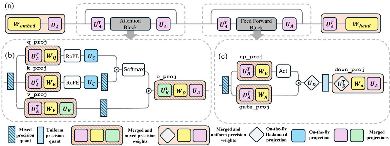
Key Engineering Trick: For \(U_D\), which operates on the hidden dimension of the FFN (which is huge), doing a full matrix multiplication is too slow. The authors smartly choose \(U_D\) to be a Hadamard matrix. Hadamard transforms can be computed using fast, specialized kernels (Fast Walsh-Hadamard Transform), making the projection almost free computationally.
Experiments & Results
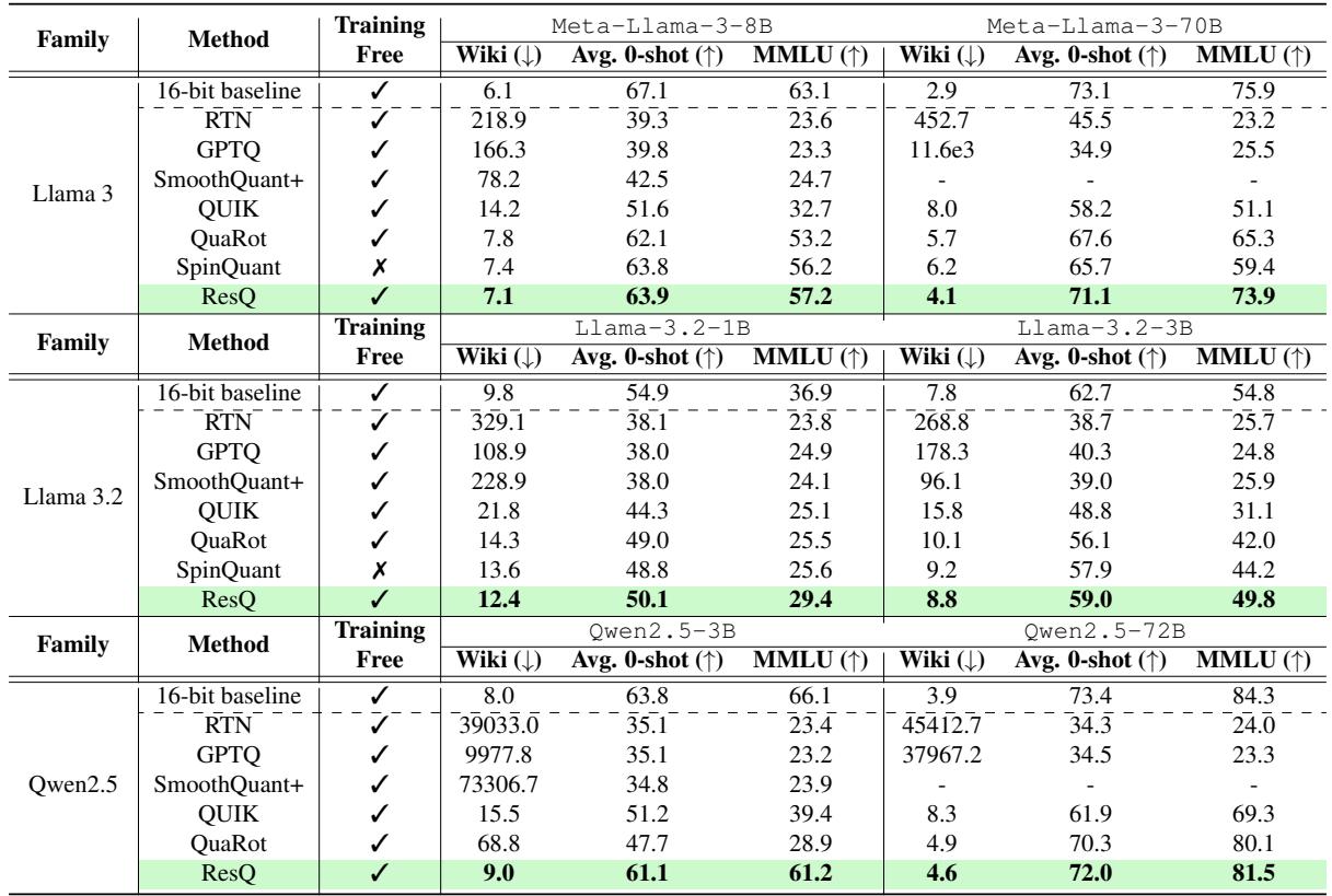
The researchers tested ResQ on Llama 2, Llama 3, Llama 3.2, and Qwen2.5 families. The setup generally quantizes Weights, Activations, and KV Cache all to 4-bit (W4A4KV4), keeping only 1/8th of the channels in 8-bit.
Perplexity and Accuracy
The results show a clear victory over competing methods like SpinQuant, QuaRot, and QUIK.
In Table 1, look at the Meta-Llama-3-70B column.
- RTN (Round-to-Nearest) breaks the model completely (perplexity > 400).
- GPTQ (Weight only) fails because activations aren’t handled.
- SpinQuant (the previous state-of-the-art) gets 6.2 perplexity.
- ResQ achieves 4.1 perplexity, significantly closer to the 16-bit baseline.
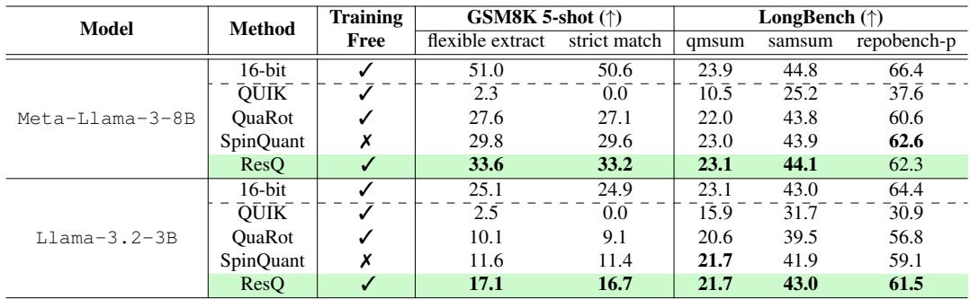
Generative Capabilities
It’s one thing to have good perplexity (predicting the next word), but can the model still do math and code?
Table 2 highlights performance on GSM8K (math) and HumanEval type tasks (code). For Llama-3-8B, ResQ scores 33.6% on GSM8K, beating SpinQuant’s 29.8% and QUIK’s 2.3% (which collapsed completely). This confirms that ResQ preserves the model’s “reasoning” abilities far better than other 4-bit techniques.
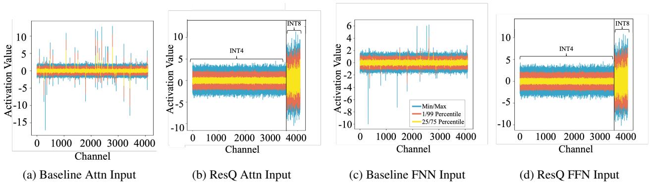
Visualizing the Improvement
To visualize why ResQ works better, we can look at the signal-to-noise ratio (SNR) and the actual activation values.
Figure 7 compares the input activations.
- Top (Baseline): The values range wildly from -15 to +10.
- Bottom (ResQ): The values are tightly controlled, mostly staying between -5 and +5. This compact range is much “friendlier” for 4-bit quantization.
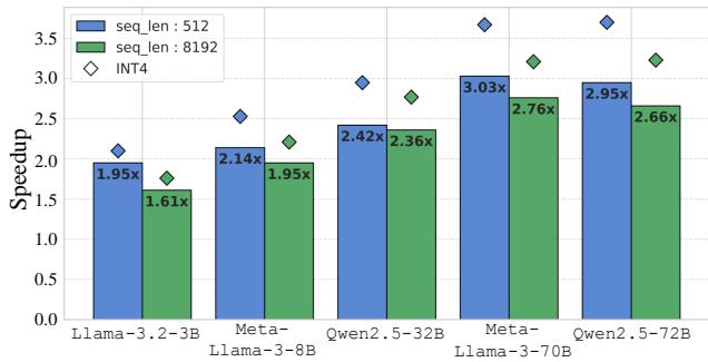
Speedup
Finally, the “Post-Training Quantization” (PTQ) promise is speed. Does ResQ deliver?
On an NVIDIA RTX 3090, ResQ achieves up to a 3x speedup over the 16-bit baseline. Crucially, it is only about 14% slower than a pure naive INT4 kernel. This means the overhead of the mixed-precision handling (splitting the matrix) and the on-the-fly projections is negligible compared to the gains from reducing memory bandwidth.
Conclusion & Implications
ResQ represents a maturation in the field of LLM quantization. We have moved past simple rounding (RTN) and static outlier clipping. We are now entering an era where quantization is “aware” of the data structure.
By mathematically separating the high-variance “signal” from the low-variance “noise” using PCA, ResQ allows us to spend our “bit budget” where it matters most.
Key Takeaways:
- Don’t just look at magnitude: Variance (PCA) is a better indicator of importance for mixed-precision than simple absolute values.
- Orthogonality is efficient: Decomposing matrices into orthogonal subspaces allows for mixed-precision without complex cross-calculations.
- Rotation aids quantization: Even after finding the best subspaces, random rotation helps smooth out the remaining outliers.
- 4-bit W/A/KV is viable: We are closing the gap to 16-bit performance, making it feasible to run massive models like Llama-3-70B on consumer-grade hardware or significantly cheaper cloud instances.
As LLMs continue to grow, techniques like ResQ that optimize the inference stage are likely to become standard components of model deployment pipelines.